


Next: 4. Density-Matrix Formulation
Up: 3. Quantum Mechanics of
Previous: 3.2 Periodic systems
Contents
Subsections
3.3 The pseudopotential approximation
In this section we outline a further approximation which is based upon the
observation that the core electrons are relatively unaffected by the
chemical environment of an atom. Thus we assume that their (large)
contribution to the total binding energy does not change when
isolated atoms are brought together to form a molecule or crystal. The actual
energy differences of interest are the changes in valence electron
energies, and so if the binding energy of the core electrons can be subtracted
out, the valence electron energy change will be a much larger fraction of
the total binding energy, and hence much easier to calculate accurately.
We also note that the strong nuclear Coulomb potential and highly localised
core electron wave-functions are difficult to represent computationally.
Since the atomic wave-functions are eigenstates of the atomic Hamiltonian,
they must all be mutually orthogonal. Since the core states are localised in
the vicinity of the nucleus, the valence states must oscillate rapidly in
this core region in order to maintain this orthogonality with the core
electrons. This rapid
oscillation results in a large kinetic energy for the valence electrons in
the core region, which roughly cancels the large potential energy due
to the strong Coulomb potential. Thus the valence electrons are much more
weakly bound than the core electrons.
It is therefore convenient to attempt to replace the strong Coulomb potential
and core electrons by an effective pseudopotential which is much
weaker, and replace the valence electron wave-functions, which
oscillate rapidly in the core region, by pseudo-wave-functions, which vary
smoothly in the core region [56,57].
We outline two justifications for this
approximation below; for further details see [58] and also
[59,60] for recent reviews.
Figure 3.2:
Schematic diagram of the relationship between all-electron and pseudo-
potentials and wave-functions.
|
|
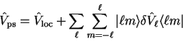
Following the orthogonalised plane-waves approach [61],
we consider an atom with Hamiltonian  , core states
 and core energy eigenvalues
  and focus on one
valence state
and focus on one
valence state
 with energy eigenvalue
  . From these states
we attempt to construct a smoother pseudo-state
. From these states
we attempt to construct a smoother pseudo-state
 defined by
 |
(3.55) |
The valence state must be orthogonal to all of the core states (which are of
course mutually orthogonal) so that
 |
(3.56) |
which fixes the expansion coefficients  . Thus
 |
(3.57) |
Substituting this expression in the Schrödinger equation
 gives
gives
 |
(3.58) |
which can be rearranged in the form
 |
(3.59) |
so that the smooth pseudo-state obeys a Schrödinger equation with an
extra energy-dependent non-local potential
 ;
;
The energy of the smooth state described by the pseudo-wave-function is the same
as that of the original valence state. The additional potential
 , whose effect is localised in the core, is repulsive and
will cancel part of the strong Coulomb
potential so that the resulting sum is a weaker pseudopotential.
Of course, once the atom interacts with others, the energies of the
eigenstates will change, but if the core states are reasonably far from
the valence states in energy (i.e.
, whose effect is localised in the core, is repulsive and
will cancel part of the strong Coulomb
potential so that the resulting sum is a weaker pseudopotential.
Of course, once the atom interacts with others, the energies of the
eigenstates will change, but if the core states are reasonably far from
the valence states in energy (i.e.
 ) then fixing
in
to be the atomic valence eigenvalue is a reasonable approximation. In fact we would like to make the behaviour of the
pseudopotential follow that of the real potential to first order in , and
this can be achieved by constructing a norm-conserving pseudopotential
(see section 3.3.3).
) then fixing
in
to be the atomic valence eigenvalue is a reasonable approximation. In fact we would like to make the behaviour of the
pseudopotential follow that of the real potential to first order in , and
this can be achieved by constructing a norm-conserving pseudopotential
(see section 3.3.3).
For a fuller discussion of the theory of scattering see [62].
Consider a plane-wave with wave-vector  scattering from some
spherically-symmetric potential
localised within a radius
scattering from some
spherically-symmetric potential
localised within a radius  and centred at the origin.
The incoming plane-wave can be decomposed into spherical-waves by the identity
and centred at the origin.
The incoming plane-wave can be decomposed into spherical-waves by the identity
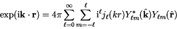 |
(3.62) |
where
 denotes a unit vector in the direction of .
These spherical- or partial-waves are then elastically scattered by the potential
which introduces a
phase-shift
denotes a unit vector in the direction of .
These spherical- or partial-waves are then elastically scattered by the potential
which introduces a
phase-shift  , which is related to the logarithmic derivative
of the exact radial solution for given
, which is related to the logarithmic derivative
of the exact radial solution for given  and energy
 within the core, evaluated on the surface of the core region:
 |
(3.63) |
 and
and  denote the spherical Bessel and von Neumann functions
respectively, and the radial wave-function
denote the spherical Bessel and von Neumann functions
respectively, and the radial wave-function  is related to the
solution of the Schrödinger equation with angular momentum state determined
by the good quantum numbers and
is related to the
solution of the Schrödinger equation with angular momentum state determined
by the good quantum numbers and  , and energy , within the core
region,
, and energy , within the core
region,
 by
by
 |
(3.64) |
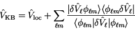
The phase-shifted spherical-waves can then be recombined to form the
total scattered wave. We can define a reduced phase-shift  by
by
 |
(3.65) |
which has the same effect (the scattering amplitude depends on
 so that factors of
  in
have no effect) and fix by requiring to lie in the
interval
in
have no effect) and fix by requiring to lie in the
interval
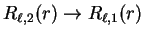
 . The integer counts the
number of radial nodes in , two in the case of figure
3.2, and is thus equal to the number of core states with
angular momentum
. The integer counts the
number of radial nodes in , two in the case of figure
3.2, and is thus equal to the number of core states with
angular momentum  .
.
The pseudopotential is then defined as the potential
whose complete phase-shifts are
the reduced shifts so that the radial pseudo-wave-function has
no nodes and thus the potential has no core states. The scattering effect
of this potential is the same as the original potential. We note again the
energy-dependence of the phase-shifts so that for a good approximation it
will be necessary to match these phase-shifts to first order in the energy
so that it is accurate over a reasonable range of energies, a property
which results in good transferability of the pseudopotential i.e. it
is accurate in a variety of different chemical environments. The non-local
nature is also exhibited since different angular momentum states are
scattered differently.
3.3.3 Norm conservation
The conditions of a good pseudopotential are that it reproduces the
logarithmic derivative of the wave-function (and thus the phase-shifts)
correctly for the isolated atom, and also that the variation of this quantity
with respect to
energy is the same to first order for pseudopotential and full potential3.2.
Having replaced the full potential by a pseudopotential, we can once again
solve the Schrödinger equation in the core region to obtain the
pseudo-wave-function, with radial part
 .
.
Pseudopotential generation has itself been the subject of a great deal of
study in the past (see [65,66,67,68,69,70,71,72,73])
and in this work we have chosen to use those pseudopotentials
generated by the method of
Troullier and Martins [74]. With one notable exception
[75], all of the recent methods have used
norm-conservation to guarantee that the phase-shifts are correct to first
order in the energy (correction to higher orders is also possible
[76]).
Consider the following second-order ordinary differential equations which
are eigenvalue equations for the same differential operator but with
different eigenvalues:
In the context of homogeneous differential equations, the quantity known as
the Wronskian is defined by
 |
(3.67) |
and can be calculated according to
![\begin{displaymath}
W(x) = W_0 \exp \left[ - \int^x {\mathrm d}x' p(x') \right]
\end{displaymath}](img357.gif) |
(3.68) |
in which the constant  is arbitrary and of no consequence.
Following a similar analysis which leads to equation 3.68 for
the quantity defined in equation 3.67 but for the functions
which solve equations 3.66 we obtain
![\begin{displaymath}
W(x) = \left[ (\lambda_2 - \lambda_1) \int^x {\mathrm d}x' y...
...+ W_0 \right] \exp \left[ - \int^x {\mathrm d}x' p(x') \right]
\end{displaymath}](img359.gif) |
(3.69) |
and note that the Wronskian can also be rewritten in terms of logarithmic
derivatives:
![\begin{displaymath}
W(x) = y_1(x) y_2(x) \frac{\mathrm d}{{\mathrm d}x}
\Bigl\{ \log[y_2(x)] - \log[y_1(x)] \Bigr\} .
\end{displaymath}](img360.gif) |
(3.70) |
Using equations 3.69 and 3.70 in the case of the
Schrödinger equation for the radial wave-function , by making the replacements
and using limits
 we obtain
 |
(3.71) |
Rearranging, multiplying by  and noting that the lower limit on the
left-hand side contributes nothing because of the
and noting that the lower limit on the
left-hand side contributes nothing because of the  factor:
 |
(3.72) |
Finally, taking the limit
 so that
 and interpreting the left-hand side as a
derivative with respect to energy we obtain the desired result:
and interpreting the left-hand side as a
derivative with respect to energy we obtain the desired result:
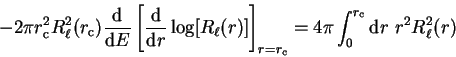 |
(3.73) |
i.e. the first energy-derivative of the logarithmic derivative evaluated at
the core radius (and hence the phase-shift) is related directly to the
norm of the radial wave-function within the core region. Thus if the
pseudo-wave-function is norm-conserving such that
 |
(3.74) |
then the phase-shifts of the pseudopotential will be the same as those of the
real potential to first order in energy, and this can be achieved by making
the pseudo-wave-function identical to the original all-electron wave-function
outside the core region.
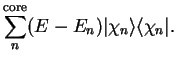
We have seen that it is necessary to use a non-local pseudopotential to
accurately represent the combined effect of nucleus and core electrons, since
different angular momentum states (partial waves) are scattered differently.
In general we can express the non-local pseudopotential in semi-local
form
 |
(3.75) |
in which
 denotes the spherical harmonic
  .
The choice of local potential
.
The choice of local potential
 is arbitrary, but in
general the sum over is truncated at a small value (e.g.
is arbitrary, but in
general the sum over is truncated at a small value (e.g.  ) so
that the local part is required to represent the potential which acts on
higher angular momentum components.
) so
that the local part is required to represent the potential which acts on
higher angular momentum components.
This semi-local form suffers from the disadvantage that it is computationally
very expensive to use, since the number of matrix elements which
need to be calculated scales as the square of the number of basis states,
and this is generally too costly. In section 5.6.1 we will
describe how this problem can be overcome analytically with a certain set of
localised basis functions, but the most common solution, and one which we
have also implemented for consistency, is to use the Kleinman-Bylander
separable form [77]
 |
(3.76) |
where
 is an eigenstate of the atomic pseudo-Hamiltonian.
This operator acts on this reference state in an identical manner to the
original semi-local operator
is an eigenstate of the atomic pseudo-Hamiltonian.
This operator acts on this reference state in an identical manner to the
original semi-local operator
 so that it is
conceptually well-justified, but now the number of projections which need to
be performed scales only linearly with the number of basis states.
This separable form can in fact be viewed as the first term of a complete
series [78].
so that it is
conceptually well-justified, but now the number of projections which need to
be performed scales only linearly with the number of basis states.
This separable form can in fact be viewed as the first term of a complete
series [78].
Next: 4. Density-Matrix Formulation
Up: 3. Quantum Mechanics of
Previous: 3.2 Periodic systems
Contents
Peter Haynes
![\begin{picture}(285,199)
\put(28,0){\includegraphics [width=8cm]{psfig.eps}}
\pu...
...{\mathrm{ps}}$}}
\put(168,111){$r_{\mathrm c}$}
\put(262,117){$r$}
\end{picture}](img314.gif)
![\begin{displaymath}x \rightarrow r \quad ; \quad
p(x) \rightarrow \frac{2}{r} \...
...r^2} \right] \quad ; \quad
\lambda \rightarrow -2E , \nonumber \end{displaymath}](img361.gif)