CASTEP contains implementations of several methods for computing the electronic response orbitals and the dynamical matrix [6]. The choice of the most suitable one depends on the type of calculation. For insulators, and particularly polar insulators the density-functional perturbation theory method (DFPT) is preferred (section 2.1), as this is not only the most efficient, but also allows the calculation of infra red and raman intensities for modelling of spectra. DFPT is not yet implemented for metallic systems or for ultrasoft pseudopotentials (as of release 4.4), and in these cases the finite displacement method may be used (section 2.4). If a density of states or finely sampled dispersion curve along high symmetry directions is needed, then either the DFPT method with Fourier interpolation (section 2.3) is the most suitable (for insulators) or the finite-displacement supercell (section 2.5; for metals or if ultrasoft pseudopotentials are required).
Many of the principles of setting up and running phonon calculations can be illustrated in the simplest case - computing phonon frequencies at the q = (0,0,0), often referred to as the Γ point. This is a very common calculation, as it forms the basis of modelling of infra-red or raman spectra and group theoretical analysis and assignment of the modes.
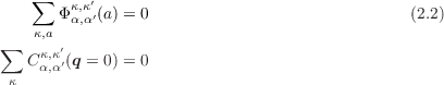
The setup for a CASTEP phonon calculation requires a few additional keywords in the seedname.cell file. Like any type of calculation, the unit cell must be specified using either of %BLOCK LATTICE_ABC or %BLOCK LATTICE_CART, and the atomic co-ordinates using %BLOCK POSITIONS_FRAC or %BLOCK POSITIONS_ABS. Figure 2.1 shows a complete input file for a calculation on boron nitride in the hexagonal Wurtzite structure. Note the additional keywords. PHONON_KPOINT_LIST is used to specify that a single phonon wavevector (0,0,0) is to be computed. More wavevectors could be specified using additional lines in this block.
Figure 2.3 shows part of the phonon-relevant output extracted from the .castep file obtained by running the input files of the previous section. There are several blocks of output, one per direction chosen for q → 0 in the LO-TO splitting terms. Note that CASTEP has added a calculation without LO-TO splitting (the first block), even though this was not explicitly requested. Within each block frequencies are listed one per line. Also on the line are (a) a label indicating the irreducible representation of the mode from a group theory analysis, (b) the computed absorptivity of the mode in a powder (or otherwise orientationally averaged) infrared experiment, (c) whether the mode is ir active, (d) the raman activity (if computed) and (e) whether the mode is raman active.
As with other calculations the amount of information written to the .castep file is controlled by the value of the parameter IPRINT. The levels of output are
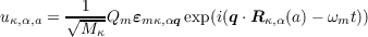
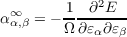
In addition to the user-readable output in the .castep file, every phonon calculation generates an additional output file with the suffix .phonon which is intended for postprocessing analysis by other programs. This includes not only the frequencies but also the eigenvectors εmκ,αq resulting from diagonalising the dynamical matrix. These eigenvectors are orthonormal by construction, and the relationship between the eigenvectors and atomic displacements is given by
|
| (2.1) |
where QM is the amplitude of mode m and the other notation is as set out in the introduction.
In addition to the infrared absorptivity computed as a default part of a Γ-point phonon calculation, CASTEP is also capable of computing the raman activity tensors in the case of nonresonant scattering. This calculation requires substantially more computational effort than a phonon calculation and is therefore not enabled by default. To compute raman activity set
in the .param file. As of CASTEP 4.4 the calculation uses a finite-difference method (see section 2.4 to compute the mode displacement derivatives of the polarizability tensor (section 2.6) using the approach of Porezag and Pedersen [7]. The first stage is to perform a full phonon calculation at q = 0, to determine the mode eigenvectors and identify the raman-active modes. Then CASTEP loops over the active modes only computing the raman tensor, activity and depolarization for each. The raman activity is printed as part of the usual frequency output given in figure 2.3.
Phonons of a nonzero wavevector play an important role in the thermophysical properties of crystalline solids and the physics of many solid-state phase transitions. Proving the mechanical stability of a crystal structure by testing for real frequencies requires a vibrational calculation over the full Brillouin Zone. And dispersion curves and densities of states are frequently required for comparison with inelastic neutron and X-ray scattering experiments.
One of the benefits of density functional perturbation theory is that CASTEP can calculate vibrational modes at q≠0 as easily as at q = 0 (but at the cost of an increase in CPU time due to the decreased symmetry). It is possible to perform this calculation simply by providing a list of q-points in the .cell file ( using one of the blocks %BLOCK PHONON_KPOINT_LIST, or %BLOCK PHONON_KPOINT_PATH or keyword PHONON_KPOINT_MP_GRID). However to generate a reasonable quality dispersion plot or density of states will usually require hundreds or thousands of q-points. The time required by such a calculation would be several hundred times that for a single-point energy and therefore infeasibly large.
Fortunately there is a way to achieve the same result at a far smaller computational cost. This method exploits the fact that the interatomic interactions in a solid have a finite range and decay rapidly to zero. Specifically, the elements of the force constant matrix in Eq. 1.2 decrease as 1∕r5 with interatomic distance. Consequently the dynamical matrix defined by Eq. 1.5 and its eigenvalues ω2(q) are smoothly varying with wavevector q. Fourier interpolation is used to generate dynamical matrices on an arbitrarily fine grid or line sample in reciprocal space from a set of DFPT calculations on a much coarser grid. For a full description of the method see references [5, 8, 1].
A complication arises in the case of polar solids where the dipole-dipole interaction generated upon displacing an atom leads to a longer ranged force constant matrix which decays only as 1∕r3. CASTEP models this term analytically using Born effective charges and dielectric permittivity calculated using an electric field response DFPT calculation (see section 2.6 and Ref. [1]). It is therefore able to perform the Fourier interpolation only for the part of the force constant matrix which varies as 1∕r5, and does not require a finer grid than in the case of non-polar solids.
In the .cell file choose the q-points of the coarse grid of points at which to perform DFPT calculations. This may be specified as a %BLOCK PHONON_KPOINT_LIST containing the reduced set of points in the irreducible Brillouin Zone, but is is almost always more straightforward to use the alternative keywords
phonon_kpoint_mp_grid p q r
phonon_kpoint_mp_offset o1 o2 o3
to specify the grid parameters and offset. The grid parameters p, q and r should normally be chosen to give a roughly uniform sampling of reciprocal space taking length of the reciprocal lattice vectors into account, and should be compatible with the symmetry of the simulation cell. Alternatively a grid may be specified using the minimum spacing, for example
phonon_kpoint_mp_grid_spacing 0.1 1/ang
Normally the grid should be chosen to contain the Γ point, which usually gives better convergence properties of the interpolation (i.e.convergence at smaller p,q,r) than otherwise. (This is the opposite of the convergence behaviour of electronic k-point sampling - see Ref. [9]). A grid with odd values of p, q and r will contain the Γ point in the absence of an offset. However if, for example p is even then setting o1 = 1∕(2p) using phonon_kpoint_mp_offset will create an even grid containing the origin in that direction.
The choice of grid parameters p, q and r will be influenced by the nature of the system under study. Ionically bonded systems tend to have fairly short-ranged force-constant matrices and need relatively coarse grids for convergence. For example, sodium chloride in the rocksalt structure with a primitive lattice parameter 3.75Å a 4 × 4 × 4 grid is reasonably close to convergence. This corresponds to a truncation of the force constant matrix at a distance greater then 7.5Å. On the other hand covalent systems tend to have fairly long-ranged force-constant matrices and need finer grids for convergence. Silicon is a good example of this. The primitive lattice parameter is similar to sodium chloride at 3.81Å, but the dispersion curve is not fully converged until an 8 × 8 × 8 grid is used. A more detailed examination of this point may be found in reference [10].
Additional keywords in the .param file control the interpolation. Most importantly
PHONON_FINE_METHOD : INTERPOLATE
instructs CASTEP to perform the Fourier interpolation step following the usual DFPT calculation.
The target set of wavevectors for the interpolation is set up using additional keywords or blocks in the .cell file.
phonon_fine_kpoint_mp_grid p q r
phonon_fine_kpoint_mp_offset o1 o2 o3
will perform interpolation onto a regular (possibly offset) grid. In fact only the points in the irreducible wedge of the Brillouin Zone are included, and a suitable weight is computed so that the weighted average is identical to a uniform sampling of the BZ. This is the usual method for computing a phonon density of states.
Alternatively if a set of dispersion curves along high symmetry directions is required, the alternative cell keyword block
%BLOCK PHONON_FINE_KPOINT_PATH
0.0 0.0 0.0
0.5 0.5 0.0
0.5 0.5 0.5
...
%ENDBLOCK PHONON_FINE_KPOINT_PATH
will set up a list traversing the directions between the points specified. The additional keyword
PHONON_FINE_KPOINT_PATH_SPACING 0.03 1/ang
can be used to set the point spacing (in reciprocal length) along the path to the physical value specified as argument. As a final alternative, a simple list of points can be generated to generate any sampling you choose using
%BLOCK PHONON_FINE_KPOINT_LIST
0.0 0.0 0.0
0.1 0.2 0.3
...
%ENDBLOCK PHONON_FINE_KPOINT_LIST
This is the approach used for files generated by Accelrys Materials Studio.
The same keywords are used in the closely related method of a supercell calculation; see the example .cell file of figure 2.4.
CASTEP stores the results of all phonon calculations - dynamical matrices and force constant matrices - in the binary seedname.check file written at the end of a successful run. This can be used to change some values of parameters relating to interpolation, and to change or indeed replace the entire fine phonon k-point set without any need to repeat the expensive DFPT (or supercell) part of the calculation. In fact a single calculation of the force constant matrix is sufficient to compute a DOS at a variety of sampling densities plus arbitrarily smooth dispersion curves.
Setting up a continuation calculation is simple. Just add the continuation keyword in the usual way to a renamed copy of the param file
continuation orig-seedname.check
and make any changes fine k-point sampling parameters in a copy of the seedname.cell file. It is recommended that you work with renamed copies to avoid overwriting the original and valuable seedname.check file. Running CASTEP on the new set of input files is exactly the same as running a new calculation, except that the result will be generated much more quickly.
When setting up a continuation run, take care not to change the standard phonon k-point set, the electronic k-point set or any electronic structure parameters such as elec_energy_tol. If a mismatch is detected with the values stored in the checkpoint file, CASTEP will discard the saved dynamical matrix data and restart the full calculation from the beginning.
The phonons program provides an alternative interface to running CASTEP itself for such continuation calculations. See section 3.4 for details.
The final representation of the Force constant matrix derived from the dynamical matrices is actually a periodic representation and is equivalent to the q = 0 dynamical matrix of a (fictitious) p × q × r supercell. (See section 2.5 for more explanation.) CASTEP must determine a mapping between elements of the periodic dynamical matrix and aperiodic force constant matrix using a minimum-image convention for ionic site pairs and impose a cutoff scheme in real space to exclude (supercell-) periodic images. In fact CASTEP implements two distinct schemes.
The cumulant scheme [11] includes all image force constants with a suitable weighting to avoid multiple counting of images. This is achieved by including image force constants in any direction if they lie within half the distance to the nearest periodic repeat of the fictitious supercell lattice in that direction. If an atom-atom pair vector lies exactly half way to the supercell repeat so that image force constants occur, for example, at both L and -L, all images at the same distance are included with a suitable weighting factor to preserve the symmetry of the cumulant force constant matrix. (See Refs. [11] and [12] for a more detailed explanation). This scheme is selected by specifying the param file keyword
and is in fact the default method in CASTEP 5.0 and later. In CASTEP versions 4.4 and earlier this method is selected by
CASTEP also implements a simple spherical cutoff, controlled by the parameter Rc and specified by parameter
The value Rc should be chosen to satisfy 2Rc < min(pL1,qL2,rL3)L where Ln is the cell edge of the simulation cell and p,q,r are the (coarse) grid of phonon wavevectors. It is usually easiest to specify a value of zero, in which case CASTEP chooses the largest allowable value automatically. This scheme is most suitable for bulk materials of cubic symmetry. The spherical scheme is chosen using keyword
in CASTEP 5.0 or later and is the default in earlier releases.
Within the default method a smaller cutoff volume can be selected by decreasing the value
of
PHONON_FORCE_CONSTANT_ELLIPSOID by a small fraction (4.4 and earlier) or by the new parameter
PHONON_FORCE_CONSTANT_CUT_SCALE (5.0 and later). This may be useful for testing the effect of
long-ranged contributions to the IFC matrix. However any departure of this parameter’s value from 1
does not preserve the superior convergence properties of the cumulant scheme and will in general require
a larger supercell than the exact cumulant method.
The vibrational Hamiltonian is invariant to a uniform translation of the system in space. This symmetry is the origin of the well-known result that any crystal has three acoustic vibrational modes at q = 0 with a frequency of zero. Any book on lattice dynamics will discuss the so-called acoustic sum rule (or ASR) which has mathematical expressions for the force constant and Γ-point dynamical matrices
In plane-wave calculations the translational invariance is broken as atoms translate with respect to the fixed FFT grid, so the sum rule is never exactly satisfied. Consequently it is sometimes observed even in an otherwise apparently very well converged calculation that the three acoustic modes at Γ depart significantly from zero frequency. Depending on the XC functional1 these frequencies may reach or exceed 50 cm-1. One solution is simply to increase the FFT grid parameters using parameter FINE_GRID_SCALE to increase the density grid and not the wavefunction grid. However this can be prohibitively costly in computer time and memory.The better solution is to apply a transformation to the computed dynamical or force constant matrix so that it exactly satisfies the ASR. CASTEP implements a scheme which projects out the acoustic mode eigenvectors and adjusts their frequency to zero, while having minimal impact on the optic mode frequencies. This scheme is controlled by parameters (in the .param file)
The first of these simply activates or deactivates the correction. The second chooses which of the variants of the ASR in equation 2.3 to enforce, the real-space force constant matrix, the reciprocal-space dynamical matrix, or both. (PHONON_SUM_RULE_METHOD : NONE is a synonym for PHONON_SUM_RULE : FALSE). The real-space method is only applicable to interpolation or supercell/finite displacement calculations, but the reciprocal-space method can be used for any type of phonon calculation.
Both variants change the acoustic mode frequencies away from but near q = 0, the realspace method implicitly, and the reciprocal space method explicitly, by determining the correction to Dκ,κ′ α,α′(q = 0) and subtracting it from Dκ,κ′ α,α′(q) as suggested by Gonze [1]. This usually results in acoustic mode behaviour which is indistinguishable from a very well converged calculation using a very fine FFT grid2 .
In addition to the sum rule on frequencies there is another for the Born effective charges (see section 2.6)
 | (2.3) |
which is activated by parameter
The default behaviour of CASTEP is that neither sum rule is enforced. If this was not requested in the original run, then it may be added in post-processing fashion in a continuation run, as per section 2.3.2. Only the raw dynamical and/or force constant matrices are stored in the checkpoint file without the effect of ASR enforcement, which is only applied at the printout stage. Therefore the effect can be turned off, or altered by a post-processing calculation as well as turned on.
In addition to the DFPT method of computing force constants, CASTEP implements schemes based on numerical differentiation of forces when atoms are displaced by a small amount from their equilibrium positions. These may be used in cases where a DFPT calculation can not, for example in calculating phonon dispersion of metallic or magnetic systems, or when the use of ultrasoft pseudopotentials is essential.
There are two variants of this scheme. The basic finite displacement method is selected by setting parameter
PHONON_METHOD : FINITEDISPLACEMENT
In contrast to DFPT such displacements are necessarily periodic with the simulation cell, and therefore only q = 0 phonons are commensurate with this condition. As in the case of DFPT lattice dynamics the phonon wavevectors are specified by %BLOCK PHONON_KPOINT_LIST, %BLOCK PHONON_KPOINT_PATH or PHONON_KPOINT_MP_GRID in the .cell file but only the Γ point, (0,0,0) is meaningful. CASTEP will print a warning in the output file and ignore any non-zero value in the list.
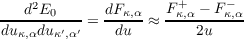
CASTEP proceeds by shifting each atom by a small amount, then performing a SCF calculation to evaluate the forces on the perturbed configuration. Both positive and negative displacements are performed in each direction so that the corresponding force constants can be evaluated using the accurate “central difference” method of numerical differentiation.
 | (2.4) |
Equation 2.4 demonstrates that a single pair of displaced calculation yields an entire row of the dynamical matrix. As with DFPT calculations, only the minimal set of perturbations is performed and the space-group symmetry is used to build the complete dynamical matrix.
The SCF calculations on the perturbed configuration are efficient, typically taking only only a few cycles in CASTEP 5.0 or later. This efficiency is achieved by first making a good guess for the electron density of the perturbed system based on the ground state of the unperturbed system, and applying a displacement of an atomic-like density of the pseudo-atom in question. Second, the SCF is started using the Kohn-Sham orbitals of the unperturbed state as the initial guess for the perturbed configuration. To exploit this efficiency it is essential to use the density-mixing (Davidson) minimiser, selected by ELEC_METHOD : DM in the .param file. (As the all-bands method has no means of initialising the density).
The default displacement used is 0.01 bohr This can be changed if necessary by setting a parameter,
in the .param file. Except for the differences discussed above, input and output formats are the same as for DFPT calculations.
The limitation of the finite displacement approach to q = 0 may be overcome by combining the method with the use of a supercell. This method, sometimes known as the “direct method” [13, Section 19.2] relies on the short-ranged decay of the force constant matrix with interatomic distance and makes the assumption that force constants for separations larger than some value, Rc are negligibly small and can be treated as zero. A supercell can be constructed to contain an imaginary sphere of radius Rc beyond which force constants may be neglected. Then the dynamical matrix of a supercell satisfying L > 2Rc is identical to the force constant matrix, i.e. Cκ,κ′ α,α′(q = 0) = Φκ,κ′ α,α′. Therefore complete knowledge of the force constant matrix to a reasonable approximation may be derived from a single calculation of the q = 0 dynamical matrix of a supercell containing several primitive cells. From this set of force constants the dynamical matrices at any phonon wavevector may be computed using equation 1.5 in exactly the same way as used in an interpolation calculation.
In a CASTEP calculation the supercell must be chosen and explicitly specified in the input files. It is defined by a matrix, which multiplies the ordinary simulation cell vectors and is specified as a 3 × 3 matrix in the .cell file of the form
This typical example using a diagonal matrix creates a supercell expanded along each lattice vector a, b and c by factor of 4.
The supercell to be used in a phonon calculation needs to be chosen with care.
The electronic Brillouin-Zone integrals for the supercell calculation use the special k-points method, which are specified in the .cell file using an separate but analogous set of keywords to those pertaining to the primitive cell sampling. Specifically,
Once the force constant matrix has been calculated using the supercell, the remainder of the lattice dynamics proceeds exactly as in the case of a Fourier interpolation calculation. The keywords controlling the interpolation scheme and cutoff radius, the fine phonon kpoint set and the acoustic sum rule enforcement work in exactly the same way. See section 2.3.1 for details.
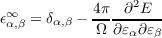
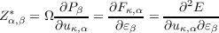
Density functional perturbation theory is not limited to atomic displacement perturbations, and may also be used to calculate other response properties with respect to an electric field perturbation4 . These are the dielectric permittivity
 | (2.5) |
the “molecular” polarizability
 | (2.6) |
and the Born effective charges
 | (2.7) |
which play a strong role in lattice dynamics of crystals, and in particular governs the frequency-dependent dielectric response in the infra-red region [1].
An electric field response calculation is selected using the task keyword in the .param file.
which computes the optical frequency dielectric permittivity tensor and the low frequency (ionic lattice) response to a time-varying field in the regime of the phonon modes and the Born charges. Alternatively
performs both dielectric and phonon tasks.
The low and near-infrared frequency contributions to the permittivity and polarizability and the Born effective charges are printed to the .castep output file. An extract for the same Wurtzite BN calculation as earlier is shown in figure 2.6. An additional output file seedname.efield is also written and contains the frequency-dependent permittivity over the entire range, with a spacing determined by parameter EFIELD_FREQ_SPACING, and a Lorentzian broadening governed by a fixed Q, EFIELD_OSCILLATOR_Q.
The low-frequency contribution of the phonons to the dielectric polarizability and permittivity is only well-defined when all mode frequencies are real and positive. In the presence of any imaginary mode or one of zero frequency the low-frequency dielectric and polarizability tensors are not calculated and are reported as “infinity”. By default the three lowest frequency modes are assumed to be acoustic modes and not included in the calculation. To support molecule-in-supercell calculations, the parameter EFIELD_IGNORE_MOLEC_MODES may be set to MOLECULE, which excludes the 6 lowest frequency modes from the dielectric calculation. Allowed values are CRYSTAL, MOLECULE and LINEAR_MOLECULE which ignore 3, 6 and 5 modes respectively.
In fact CASTEP usually performs an electric field response calculation even for a task : PHONON calculation because the permittivity tensor and Born charges are required to calculate the LO/TO splitting terms. Conversely a pure task : EFIELD calculation also performs a Γ-point phonon calculation which is needed to compute the ionic contribution to the permittivity and polarizability. Consequently the only real difference between any of the tasks PHONON, EFIELD and PHONON+EFIELD lies in what is printed to the output file as the same computations are performed in each case. Only if one or other of those properties is specifically turned off with one of the parameters
is a “pure” phonon or efield calculation ever performed.
It is well documented that the LDA tends to overestimate dielectric permittivities - by over 10% in the case of Si or Ge [14]. It is possible to include an ad-hoc correction term to model the missing self-energy, by applying the so-called “scissors operator”, which consists of a rigid upshift of all conduction band states. This was incorporated into DFPT electric field response calculations by Gonze and Lee [1]. The parameters keyword
is used to model the effect of a 1 eV (in this example) upshift of conduction band states and will include the effects on dielectric permittivity and Born charges (but not phonons). The value to use must be determined from high-level calculations or empirically.
One of the important motivations for lattice dynamical calculations of crystalline solids is that the harmonic approximation gives access to thermodynamic properties including the zero-point energy and the free energy as a function of temperature. CASTEP lattice dynamics calculations can be followed by a thermodynamics calculation to calculate the zero-point energy and temperature dependent free energy
![[ ( )]
F = Eelec + kBT ∑ ln 2sinh ℏωq,i
q,i kBT](Castep_Phonons21x.png) | (2.8) |
The thermodynamics calculation follows a previous phonon calculation. It is selected by setting the parameter
This may be used in a continuation run from a previous phonon calculation, where the value of the continuation parameter is the name of the previous .check file. Alternatively it may be configured as a new run from scratch by setting the remainder of the parameters exactly as if this were a phonon task, and the phonon calculation will be performed first. Only the phonons defined on the “fine” set of phonon kpoints will be used to compute the free energy as it is normally expected that a thermodynamics calculation will follow an interpolation or supercell calculation. However provided that the standard and fine sets of phonon k-points are identical, it may also be used following a standard phonon calculation.
This task will compute and print the free energy in the range of temperatures specified by the parameters THERMO_T_START and THERMO_T_STOP. The number of temperatures is set by one or other of the parameters THERMO_T_SPACING or THERMO_T_NPOINTS. It is almost always essential to explicitly specify the unit of K for the above temperature parameters. Due to a restriction in the input parser these are treated as energies and the default units are Hartree. The results of the calculation are written to the .castep file.
The harmonic approximation free energy is only defined if all frequencies are greater than or equal to zero. Any zero or imaginary frequencies are automatically omitted from the calculation and a warning message is printed. It is the responsibility of the end user to check that the computed free energy is not rendered meaningless by the presence of an imaginary mode.
Phonon and dielectric response calculations give rise to a number of issues with convergence, in addition to those encountered in ground-state calculations, and a systematic and step-by-step approach is necessary to achieve well-converged results. CASTEP assists the user by setting default values for many convergence parameters based on the particular task which incorporate the experience of many calculations. Therefore it is a good practice not to specify convergence parameters explicitly unless specific convergence test results are known - otherwise a well-chosen default could be overridden with an untested value. (The example input of figure 2.2 contains no phonon-specific convergence parameters.)
It was emphasised previously (section 1.2.1) that a well-converged geometry optimisation is a prerequisite for a phonon calculation. In turn this mandates a reasonably high level of convergence of plane-wave cutoff, SCF convergence and electronic k-point sampling. It is typical to run phonon calculations at a BASIS_PRECISION : FINE level of plane-wave cutoff, (The header of each .usp or .recpot pseudopotential file contains a translation into eV units.) DFPT electric field response calculations can require finer electronic k-point sampling than suffices for a ground state calculation, so the effect of the KPOINT_MP_GRID on the dielectric permittivity should be tested.
The second stage of a phonon or efield calculation is the variational DFPT solver, and there are a number of associated parameters to control the convergence. Parameters
and
govern the exit criterion for the DFPT self-consistency loop. The above default values are usually sufficient for frequencies converged to < 1cm-1 and permittivities to two or three decimal places and rarely need to be changed.
However the converged results depend not only on the DFPT SCF calculation, but also, and rather strongly on the degree of convergence of the ground state electron density and wavefunctions. The ground-state wavefunctions enter the DFPT equations both directly and as a consequence of the orthogonality condition between ground-state and first-order response orbitals [6, 1]. Specifically, the error in the second-order energy or force constants is variational, and therefore depends quadratically on the error in the DFPT first-order response orbitals. However it is non-variational and linear with respect to the error in the ground-state orbitals. The practical consequence is that there is an error in DFPT results which varies as the square root of the ground-state convergence parameter ELEC_ENERGY_TOL which therefore must be very small for good accuracy. A heuristic rule of thumb is that ELEC_ENERGY_TOL ≈PHONON_ENERGY_TOL2 is necessary to converge the second order energy to the value of PHONON_ENERGY_TOL. The default setting of ELEC_ENERGY_TOL is based on this heuristic and should only be changed after careful testing of the effect on frequencies or dielectric properties.
The criteria for choosing the “ground-state” convergence parameters for a finite-displacement phonon calculation (in either primitive or supercell mode) are naturally almost identical to those governing DFPT calculations. In this case there is no additional self-consistent electronic calculation; instead there is a sequence of additional ground-state calculations at displaced geometries.
Finite-displacement calculations require very well converged forces to be computed in the ground state SCF calculation. This is because the numerical evaluation of the second derivative depends on differences between the (small) forces at perturbed configurations (equation 2.4). Clearly the numerical derivative has lower relative precision than the argument (the forces), which must therefore be evaluated to a rather high precision. Unlike the ground-state energy, which is variational with respect to the orbitals, the forces are not and the error in the forces is linear in the error in the orbitals. The main parameter governing their accuracy is again
which is again set by default from the value of PHONON_ENERGY_TOL2.
It is normally sufficient to use the default value of ELEC_ENERGY_TOL chosen as the default in a phonon calculation. However there is also a way of directly achieving the requested force tolerance, by setting parameter
This is not used by default as it adds some overhead to the SCF calculation resulting in longer run times. However it does guarantee that the forces really are converged to the required accuracy, unlike setting ELEC_ENERGY_TOL.
Fourier interpolation and supercell calculations add yet another criterion which must be satisfied to achieve well-converged results - the range of the force-constant matrix in real space. Sections 2.3.1 and 2.5 discuss some of the criteria applicable to these types of calculation.
Unfortunately convergence testing of the size of the supercell for FD/supercell calculations can be prohibitively expensive as the the volume and number of atoms increase as the cube of the linear dimension under test. Consequently the CPU time will increase with the sixth power or higher! There is no easy solution to this problem and the reader is cautioned not to necessarily take on trust that FD/supercell phonon calculations published in the literature are fully converged!
However some progress may be made by performing a calculation using the largest feasible supercell. If
is selected, it is then possible to vary the cutoff radius using parameter
to lower values than the maximum of half the largest box size. These tests may be performed using the “continuation” method (section 2.3.2) or the “phonons” utility (section 3.4) without repeating the expensive supercell calculation.
Another convergence test is automatically performed if the spherical cutoff method is selected. The frequencies resulting from the interpolation with the spherical cutoff are compared to those from an “exact” interpolation at wavevectors commensurate with the supercell. The results are written to the .castep file. This provides a quantitative measure of the interpolation error.
A similar cutoff scaling test might be possible for the PHONON_FINE_CUTOFF_METHOD : DEFAULT case, although it is considerably less useful. Parameter
will scale the range of the cutoff by the factor specified. However the default value of 1.0 is “special” in including constants separated by exactly half the supercell Wigner Seitz cell. Consequently convergence is not smooth in this parameter and while 0.95 might be underconverged, 1.0 could be very well converged. (This is also the reason for its superior convergence performance over the spherical cutoff scheme.)