Dynamics
Molecular dynamics (MD) involves the stepwise integration of Newton's equations from a given starting point. It is the most natural method of performing equilibrium statistical-mechanical calculations using a simulation. Additionally, MD may be used to explore conformations, such as molecular adsorption sites on a surface. If frictional forces are added to the equations of motion, Langevin dynamics becomes possible, as does geometry optimization using damped MD. Finally, extended Lagrangian methods allow thermostatic control of the temperature.
Molecular dynamics in total-energy DFT schemes is implemented in essentially the same way as in conventional forcefield based methods. The main difference is that the energy and atomic forces are derived by solving DFT equations rather than from empirical potentials of interatomic interactions. Electrons are kept on the Born-Oppenheimer surface by means of explicit electronic structure optimization after each MD step. A side effect of this is that evaluation of force and energy from first principles is always the most computationally expensive part of ab initio MD. As a result, the efficiency of the MD step itself has no impact on the speed of the calculation.
MD in CASTEP is based on the velocity Verlet algorithm for integration of the equation of motion. The default time step can be as high as 1 fs with this algorithm because of its numerical stability and the conservation of the constant of motion.
The efficiency of the method is due in large part to the introduction of wavefunction extrapolation between MD steps (Arias et al., 1992). In addition, charge density extrapolation (Alfe, 1999) has been introduced.
Wavefunctions and density extrapolation
The main idea behind the interpolation schemes is to provide a good starting model of the electronic structure for the SCF optimization, after the geometry change. This can be achieved by using the multi-linear extrapolation as proposed by Arias et al. (1992).
The problem with wavefunction interpolation is that wavefunctions may be multiplied by an arbitrary phase factor or ordered in different ways in two contiguous steps. So, before the extrapolation is performed, the two subspaces {ψn,k(t)} and {ψn,k(t-dt)} are aligned so that Σn,k|ψn,k(t)-ψn,k(t-dt)| is minimized.
Then the wavefunctions at the next time step, t+dt, can be written as:

and similarly for the charge density:

The coefficients α and β are calculated by determining the best quadratic extrapolation of the atomic positions. This extrapolation scheme not only speeds up the calculation but also improves conservation of the constant of motion and dramatically reduces the "electronic drag" effect (Payne et al., 1992).
An improvement suggested by Alfe (1999) recognizes the fact that the charge density is mostly determined by the superposition of the atomic charge densities. Therefore one can write:

where ρ(t) is the self-consistent charge density at time t, and ρat(t) is the sum of the atomic charge densities. The charge at time t+dt is simply extrapolated as:

where the change of δρ is given by:

The atomic charge density can be calculated exactly and cheaply using the same methods as for Mulliken population analysis. The resultant scheme includes extrapolation of wavefunctions using Eq. CASTEP 31, extrapolation of charge density difference using Eq. CASTEP 35 and recalculation of the atomic charge densities.
Experience shows that the second-order extrapolation scheme described above is not necessarily the best or the fastest algorithm. CASTEP therefore offers a selection of extrapolation schemes that differ in the way the coefficients are selected: 1st order extrapolation with variable coefficients; 2nd order extrapolation with variable coefficients; alternating first and second order extrapolation steps with variable coefficients; and similar combinations of 1st and 2nd order schemes with fixed coefficients. The actual setting is controlled by the values of the MD_EXTRAP and MD_EXTRAP_FIT keywords in the .param file. The fixed coefficient scheme is based essentially on a Taylor expansion, while the variable coefficients schemes are based on the best fit between extrapolated and MD-predicted atomic coordinates. It has been shown that the accuracy of wavefunction extrapolation improves greatly when the coefficients are chosen based on the extrapolation of atomic coordinates.
An alternative to using wavefunction extrapolation is to use extended Lagrangian formulation, XL-BOMD (Steneteg 2010, Niklasson 2011) . The XL-BOMD scheme allows simultaneous propagation of nuclear and electronic degrees of freedom and shows good energy conservation at time steps that are unusually high for first principles calculations.
Ensembles
Integrating Newton's equations of motion allows you to explore the constant-energy surface of a system. However, most natural phenomena occur under conditions where the system is exposed to external pressure and/or exchanges heat with the environment. Under these conditions, the total energy of the system is no longer conserved and extended forms of molecular dynamics are required.
Several methods are available for controlling temperature and pressure. Depending on which state variables (the energy E, enthalpy H (that is, E +PV), number of particles N, pressure P, stress S, temperature T, and volume V) are kept fixed, different statistical ensembles can be generated. A variety of structural, energetic, and dynamic properties can then be calculated from the averages or the fluctuations of these quantities over the ensemble generated.
Both isothermal (where heat is exchanged with a temperature bath to maintain a constant thermodynamic temperature) and adiabatic (where no heat exchange occurs) ensembles are available:
Table 1. Thermodynamic ensembles handled by CASTEP
| Ensemble |
|---|
| Constant temperature, constant pressure (NPT) |
| Constant energy, constant volume (NVE) |
| Constant pressure, constant enthalpy (NPH) |
| Constant temperature, constant volume (NVT) |
NVE ensemble
The constant-energy, constant-volume ensemble (NVE), also known as the microcanonical ensemble, is obtained by solving the standard Newton equation without any temperature and pressure control. Energy is conserved when this (adiabatic) ensemble is generated. However, because of rounding and truncation errors during the integration process, there is always a slight fluctuation, or drift in energy.
True constant-energy conditions (that is, without temperature control) are not recommended for the equilibration phase of the simulation because, without the energy flow facilitated by temperature control, the desired temperature cannot be achieved.
However, during the data collection phase, if you are interested in exploring the constant-energy surface of the conformational space, or if for some other reason you do not want the perturbation introduced by temperature- and pressure-bath coupling, this is a useful ensemble.
Nosé NVT dynamics
The Nosé thermostat (Nosé, 1984) generates deterministic dynamics, with the temperature controlled by a fictitious additional coordinate, s, added to the Lagrangian of the system. The thermostat employs a feedback loop between the instantaneous kinetic energy and the required temperature. The rate of feedback is determined by the mass parameter, Q. This parameter should be chosen so that the natural oscillation frequency of the Nosé coordinate is close to the characteristic frequency of the actual system.
The mass parameter is related to the thermostat relaxation time by:

Where:
g is the number of degrees of freedom (usually 3N - 3, where N is the number of atoms)
kB is the Boltzmann constant
T
is the thermostat temperature
τ is the relaxation time.
An improvement on the standard Nosé thermostat (or Nosé-Hoover thermostat) is the Nosé-Hoover chain method, described in detail by Tuckerman et al. (2001). In this method the kinetic energy fluctuations of the thermostat variable are controlled by coupling it to another thermostat variable. The kinetic energy fluctuations of the second thermostat are, in turn, controlled by coupling to a third thermostat, and so on, to form a chain of M thermostats. This new coupling (the Nosé-Hoover "chain" thermostatting mechanism) leads to a more general canonical dynamics method.
Langevin NVT dynamics
The Langevin thermostat generates stochastic dynamics using a Brownian motion model, implemented using the fluctuation-dissipation theorem. It is controlled by the damping time parameter, which controls the rate of decay of fluctuations in the temperature. In practice, this should be chosen such that it is larger than the time scale of any motions of interest. An advantage of the Langevin description is that it can be proved to provide ergodic results. The Nosé thermostat, on the other hand, provides good short term dynamics, but fails to give ergodicity.
Nosé-Hoover-Langevin thermostat
The Nosé-Hoover-Langevin (NHL) thermostat suggested by Leimkuhler et al. (2009) combines the advantages of the Nosé-Hoover chain method with the ergodicity of Langevin dynamics. In practical terms this thermostat converges to equilibrium faster than the Nosé-Hoover chain method and offers much better conservation of the constant of motion.
NPT ensemble
The constant-temperature, constant-pressure ensemble (NPT) allows control over both the temperature and pressure. The unit cell vectors are allowed to change, and the pressure is adjusted by adjusting the volume of the unit cell.
Pressure is currently controlled in CASTEP using either the Andersen or Parrinello-Rahman method.
Only the size, and not the shape, of the unit cell can be changed with the Andersen method.
Temperature can be controlled using either the Nosé or the Langevin thermostat.
NPT is the ensemble of choice when the correct pressure, volume, and densities are important in the simulation. This ensemble can also be used during equilibration to achieve the desired temperature and pressure, before changing to the constant-volume or constant-energy ensemble when data collection starts.
Andersen method of pressure control
In the Andersen (1980) method of pressure control, the volume of the cell can change, but its shape is preserved by only allowing the cell to change isotropically.
The Andersen method is useful for liquid simulations since the box could become quite elongated in the absence of restoring forces if the shape of the cell were allowed to change. A constant shape also makes the dynamics analysis easier.
However, this method is not very useful for studying materials under anisotropic stress or undergoing phase transitions, which involve changes in both cell lengths and cell angles (in these situations, the Parrinello-Rahman method should be used where available).
The basic idea is to treat the volume V of the cell as a dynamic variable in the system. The Lagrangian of the system is modified so that it contains a kinetic energy term with a user-defined mass M and a potential term which is the pV potential derived from an external pressure Pext acting on volume V of the system.
Parrinello-Rahman method of pressure and stress control
The Parrinello-Rahman method of pressure and stress control can allow simulation of a structure under externally applied stress. This is useful for studying the stress-strain relationship of materials. Both the shape and the volume of the cell can change, so that the internal stress of the system can match the externally applied stress.
The method is discussed in more detail in Parrinello and Rahman, 1981 and is only summarized here.
The Lagrangians of the system are modified such that a term representing the kinetic energy of the cell depends on a user-defined mass-like parameter W. An elastic energy term pΩ is related to the pressure and volume or the stress and strain of the system. The equations of motion for the atoms and cell vectors can be derived from this Lagrangian. The motion of the cell vectors, which determines the cell shape and size, is driven by the difference between the target and internal stress.
With hydrostatic pressure only:

Where:
h={a•b•c} is the cell vector matrix
G=h'h
ri=hsi
ϕ is the interaction potential
Ω is the volume of the cell
Tr is the trace of a matrix
The dots above some symbols indicate time derivatives and the primes indicate matrix transposition.
With stress, the elastic term pΩ is replaced by:

Where:
S is the applied stress
Ω0 is the initial volume
ε is the strain
ε is also a
tensor, defined as:

It is the user-defined variable W, which determines the rate of change of the volume/shape matrix.
A large W means a heavy, slow cell. In the limiting case, infinite W reverts to constant-volume dynamics. A small W means fast motion of the cell vectors. Although that may mean that the target stress can be reached faster, there may not be enough time for equilibration.
NPH ensemble
The constant-pressure, constant-enthalpy ensemble (Andersen, 1980) is the analogue of constant-volume, constant-energy ensemble, where the size of the unit cell is allowed to vary.
Constraints
CASTEP supports linear constraints defined using the matrix Aij:

The summations are over Ni ions and Nc constraints. Vector Ri is the Cartesian position of the ith atom and C is a constant. These constraints can be used to, for example:
- Fix some of the Cartesian coordinates of the atom
- Fix the x-separation between a pair of atoms
- Constrain an atom to lie in a plane
- Constrain the center of mass to be fixed
Example
The example below (Figure 1) shows the results of an NVE calculation for a nitrogen diatomic molecule with using a time step of 1 fs. The energy conservation is excellent, the energy drift over 500 steps (0.5 ps) is less than 0.1 kcal/mole. The power spectrum of the trajectory gives the vibrational frequency as 2340 cm-1, which is within 1% of the experimental value of 2360 cm-1.
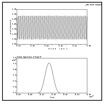
Figure 1. Bond length of the N2 molecule and power spectrum of the trajectory