Constraints

User Constraints

Any combination of linear constraints can be specified in the cell file.

We assign the index $k$ to run over all $N_{s}$ species present in the cell, the index $j$ to run over the $N_{k}$ ions in each species, and the index $i$ to run over the three spatial co-ordinates of an ion. The $y$ co-ordinate of the 2nd ion in the 3rd species is then $r_{ijk}=r_{223}$. Associated with each of these degrees of freedom is a co-efficient $a_{ijk}$. The n$^{th}$ linear constraint can then be specified as

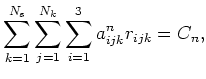$$\sum_{k=1}^{N_{s}}\sum_{j=1}^{N_{k}}\sum_{i=1}^{3}a^{n}_{ijk}r_{ijk} = C_{n},$$ (2.7)

where the constant $C_{n}$ is determined by the initial conditions. Specification of the n$^{th}$ linear constraint therefore reduces to specification of the co-efficients $a^{n}_{ijk}$. These are input into the cell file in the following fashion.

%BLOCK IONIC_CONSTRAINTS
1 S j $a^{1}_{1jk}$ $a^{1}_{2jk}$ $a^{1}_{3jk}$
1 S j $a^{1}_{1jk}$ $a^{1}_{2jk}$ $a^{1}_{3jk}$
2 O j $a^{2}_{1jk}$ $a^{2}_{2jk}$ $a^{2}_{3jk}$
2 O j $a^{2}_{1jk}$ $a^{2}_{2jk}$ $a^{2}_{3jk}$
2 O j $a^{2}_{1jk}$ $a^{2}_{2jk}$ $a^{2}_{3jk}$
%ENDBLOCK IONIC_CONSTRAINTS

For two constraints, one involving two sulfur ions, and another involving three oxygen ions. All coefficients not specified are assumed to be zero.

The first column in the block gives a unique number to the constraint specified. The second specifies the species by either atomic symbol (S or O in the above example) or atomic number. The third column is the index within a species $j$. The co-efficients of the three spatial co-ordinates for this ion under the current constraint are then specified.

As an example, let us consider the case of restricting a single ion to move along along a plane parallel to $y=x$. The normal to this plane is $\left(-1,1,0\right)$ and our constraint is that the dot product of this normal with the position vector of the ion in question is zero. If this is the second ion in the fourth species then

$$\left(-1,1,0\right)\cdot\left(r_{124},r_{224},r_{324}\right) = 0$$ (2.8)

In this trivial example, we can see that we need (if the fourth species is say, sulfur)

%BLOCK IONIC_CONSTRAINTS
1 S 2 -1 1 0
%ENDBLOCK IONIC_CONSTRAINTS

to satisfy the above equation. We shall see an example of using multiple linear constraints in section 4.1.3.

A variety of constraints can be specified in this fashion. For simplicity, a special cell file keyword is provided to fix the centre of mass in the MD calculation.

fix_com = true

This is particularly useful for Langevin dynamics simulations of small numbers of atoms. Such simulations exhibit a wandering centre of mass (with no net resultant drift) if the centre of mass is not constrained.

For calculations in the NPH or NPT ensembles, it is possible to fix the positions of all ions and hence only conduct dynamics for the cell degrees of freedom using the following.

fix_all_ions = true

Similarly, it is possible to specify that all cell degrees of freedom remain fixed.

fix_all_cell = true

It is however advisable to work in a fixed cell ensemble instead. Fixing both the cell and ionic degrees of freedom in this way will eliminate all motions and will hence return an error.

Non-linear constraints, such as those used to fix the distance between two ions, are not yet supported. Constraints on individual cell degrees of freedom are also not yet supported.

Symmetry Constraints

Many systems that are studied using CASTEP exhibit one or more symmetries. The operations defining a symmetry can be manually specified as a combination of a translation plus a rotation in the cell file. For example:

%BLOCK SYMMETRY_OPS
 0.00000000000   1.00000000000   0.00000000000
-1.00000000000   0.00000000000   0.00000000000
 0.00000000000   0.00000000000   1.00000000000
 0.75000000000   0.25000000000   0.75000000000
%ENDBLOCK SYMMETRY_OPS

This represents an application of the rotation matrix

$$\left( \begin{array}{ccc} 0&1&0 \\ -1&0&0 \\ 0&0&1 \end{array} \right)$$

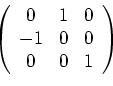
followed by a translation (in the basis of the cell vectors) of

$$\left(\frac{3}{4},\frac{1}{4},\frac{3}{4}\right).$$

Any symmetries specified in this way will generate an extra constraint to the molecular dynamics. Only motions which preserve the specified symmetry operation(s) will be permitted.

It is also possible to automatically generate all symmetry operations present using the keyword

symmetry_generate

in the cell definition file. In this case all identified symmetry operations will be preserved by the dynamics.

Symmetry constraints are not currently supported in variable cell ensembles.