Ensembles

The following statistical ensembles can be simulated using CASTEP.

NVE

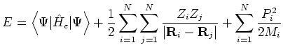
In this ensemble the shape and size of the simulation cell remain constant as specified in the cell file. The conserved energy is the Born-Oppenheimer Hamiltonian

$$E = \left<\Psi\vert\hat{H}_{e}\vert\Psi\right> + \frac{1}{2} \su... ...ert\mathbf{R}_{i}-\mathbf{R}_{j}\vert} +\sum_{i=1}^{N}\frac{P_{i}^{2}}{2M_{i}}$$ (2.1)

in atomic units.

This ensemble is selected using the command

     md_ensemble  =  nve

in the parameters file. The actual value of the conserved energy will be the result of the initial self-consistent DFT calculation plus the kinetic energy of the initial ionic velocities.

These ionic velocities are defined in one of three ways.

• By explicit user definition of ionic velocities in the cell file, e.g.

  %BLOCK IONIC_VELOCITIES 
  auv                    
  H  xxxxx yyyyy zzzzz
  H  xxxxx yyyyy zzzzz
  O  xxxxx yyyyy zzzzz 
  %ENDBLOCK IONIC_VELOCITIES
  

• By definition of an initial temperature in the parameters file, e.g.

  md_temperature  =  293 K
  

  Note that this can be specified using any valid unit of temperature. In this case initial velocities are assigned randomly such that the total linear momentum is zero and the instantaneous temperature matches that specified. The system will reach an equilibrium with a somewhat different temperature.

• By continuation from an equilibrated run at the desired temperature. This could be a run in any of the other available ensembles. This will also use the cell and ionic positions from the continuation file. See the section on continuation for details.

Velocities read from a continuation file will always take precedence. If no continuation file is used, and both md_temperature and an IONIC_VELOCITIES block are specified, the md_temperature keyword will be ignored.

By default, pressure is not calculated during an NVE run. To override this use the command

     calculate_stress = true

in the parameters file.

NVT

This ensemble is selected with

     md_ensemble  =  nvt

The system will be evolved to a specific temperature defined using the md_temperature keyword as used above. Initial velocities are assigned based on this temperature, read from an IONIC_VELOCITIES block in the cell file, or read from a continuation file in the same way as above.

Temperature control can be implemented by one of two methods, both of which have been shown to correctly sample the canonical ensemble. The first of these is the Nosé-Hoover chain method of Tuckerman et al [7] and is selected with

     md_thermostat  =  nose-hoover

in the parameters file. In the NVT case, a single Nosé-Hoover chain is coupled to all particle degrees of freedom. The length of the chain can also be specified, e.g.

     md_nhc_length  =  5

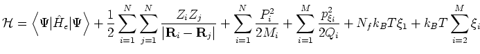
for a chain of five thermostats. In the Nosé-Hoover case with a chain of $M$ thermostats acting of $N_{f}$ ionic degrees of freedom, the conserved quantity is the pseudo-Hamiltonian

$$\mathcal{H} = \left<\Psi\vert\hat{H}_{e}\vert\Psi\right> + \frac{... ...ac{p_{\xi_{i}}^{2}}{2Q_{i}} + N_{f}k_{B}T\xi_{1} + k_{B}T\sum_{i=2}^{M}\xi_{i}$$ (2.2)

where the $Q_{i}$ are the thermostat fictitious masses assigned automatically from the specified ion relaxation time and $\xi_{i}$ are the thermostat degrees of freedom. This is printed with the label ``Hamilt Energy:'' at each time-step.

The second method of controlling temperature is the Langevin thermostat.

     md_thermostat = langevin

In this case the printed Hamiltonian energy is the value of equation 2.1. This is not conserved by the dynamics, but should exhibit no long term drift from the equilibrium value.

With either method, a suitable relaxation time for the thermostatic process should be specified. This can use any supported unit of time, e.g

     md_ion_t = 2.4 ps

for a thermostat relaxation time of 2.4 picoseconds.

As with the NVE ensemble, pressure is not calculated by default. This is overridden in the same way as the NVE case.

NPH

In this ensemble the size and (if desired) shape of the simulation cell varies to regulate pressure. No thermostat is applied.

This ensemble is specified with the following:

     md_ensemble = nph

The external pressure is set in the cell definition file using any valid unit of pressure. The required symmetry of the external pressure tensor implies that only the upper triangular components need be specified, e.g.

     %block external_pressure
     GPa
     0.5   0.0  0.0
           0.5  0.0
                0.5
     %endblock external_pressure

to specify an isotropic external pressure of 0.5 Giga-Pascals. Note that MD currently supports only isotropic external pressure. Off-diagonal components are therefore ignored.

Velocities are assigned such that the initial temperature is equal to md_temperature, or are read from the cell definition file/continuation file as in the NVE/NVT cases.

Two barostat schemes are available. The first restricts the dynamics of the cell to isotropic expansions and contractions. This follows the method of Andersen[2] and Hoover[5,6] as corrected by Martyna et al.[8]. This is selected using:

     md_barostat = andersen-hoover

In this case the printed Hamiltonian energy is the enthalpy, plus the kinetic energy associated with the cell motion.

$$H = \left<\Psi\vert\hat{H}_{e}\vert\Psi\right> + \frac{1}{2} \su... ...vert} +\sum_{i=1}^{N}\frac{P_{i}^{2}}{2M_{i}} + P_{ext}V + p_{\epsilon}^{2}/2W$$ (2.3)

The alternative scheme implements the method of Parrinello and Rahman [10,11]. Both the size and shape of the simulation cell are allowed to vary. The issue of cell rotations is eliminated by the use of a symmetrised pressure tensor. Note that as liquids cannot sustain shear, this method should only be used with solids. It should also be noted that this scheme is based on the modified Parrinello-Rahman method of Martyna, Tobias and Klien [8] which is modularly invariant, exactly obeys the appropriate tensorial virial theorem, but is only applicable to hydrostatic pressure.

The following line in the parameters file selects this barostat.

     md_barostat = parrinello-rahman

The cell dynamics contain nine degrees of freedom (of which six are independent) leading to a Hamiltonian energy of

$$H = \left<\Psi\vert\hat{H}_{e}\vert\Psi\right> + \frac{1}{2} \su... ...i}^{2}}{2M_{i}} + P_{ext}V + \mathrm{Tr}[{\mathbf{p}_{g}\mathbf{p}_{g}^{T}]}/2W$$ (2.4)

For both schemes, a relaxation time for the cell motions should be specified with an appropriate unit of time, for example:

     md_cell_t = 20 ps

This time is used to calculate a fictitious mass $W$ for the cell dynamics.

The NPH equations of motion require that pressure is calculated at each MD time-step. The value of calculate_stress is therefore irrelevant in this case.

A variable cell implies variable reciprocal lattice vectors which has consequences for the plane-wave basis set. As the cell changes, the number of plane waves required to produce the specified cut-off energy changes.

The user therefore has two options. The first is to fix the size of the basis set.

     fixed_npw = true

The cut-off energy is now variable as is the quality of the basis set. This option should therefore only be used for calculations in which the volume changes are small and which are over converged with respect to the number of plane waves.

The second option is to change the basis set at each time-step.

     fixed_npw = false

This keeps the cut-off energy approximately constant by adding or subtracting plane waves from the basis set at each time-step.

In either case, the effect of Pulay stress is reduced by applying a finite basis set correction to the pressure at each time-step. In the case of a fixed number of plane waves, the constant correction to energy is ignored. With variable number of plane waves the energy correction is no longer constant and is recalculated at each step. More details on finite basis set corrections can be found in 2.6.

Note that not all exchange-correlation functionals can be used with variable cell calculations. The choice is limited to LDA and GGA schemes only.

NPT

The NPT ensemble is specified with the command:

     md_ensemble = npt

Any combination of the thermostat and barostat schemes listed above is allowed, and is implemented in a dedicated routine. In all cases the dynamics can be shown to correctly sample the isothermal-isobaric ensemble [8,12].

All options pertaining to the NPH and NVT ensembles apply.

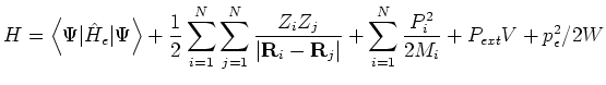
In the case of Langevin dynamics at NPT, the printed Hamiltonian energy is the same as in the NPH ensemble, i.e. that given by equation 2.3 or 2.4. In the case of Nose-Hoover NPT molecular dynamics, the Hamiltonian energy is given by

$$H = \left<\Psi\vert\hat{H}_{e}\vert\Psi\right> + \frac{1}{2} \su... ... \sum_{i=1}^{M}\frac{p_{\xi_{bi}}^{2}}{2Q_{bi}} + k_{B}T\sum_{i=1}^{M}\xi_{bi}$$ (2.5)

in the case of isotropic cell dynamics, or

$$H = \left<\Psi\vert\hat{H}_{e}\vert\Psi\right> + \frac{1}{2} \su... ...ac{p_{\xi_{bi}}^{2}}{2Q_{bi}} + 9k_{B}T\xi_{b1} + k_{B}T\sum_{i=2}^{M}\xi_{bi}$$ (2.6)

in the Parrinello-Rahman case. Note that in each case the motion of the cell degree(s) of freedom couple to a second Nosé-Hoover chain.