Predicting the thermodynamic properties of germanium
Purpose: Introduces the use of CASTEP for calculating linear response
and thermodynamic properties.
Modules: Materials Visualizer, CASTEP
Time: 
Prerequisites: Predicting the lattice parameters of AlAs from first principles
Background
Linear response, or density functional perturbation theory (DFPT), is one of the most popular methods of ab initio calculation of lattice dynamics. However, potential applications of the method extend beyond the study of vibrational properties. Linear response provides an analytical way of computing the second derivative of the total energy with respect to a given perturbation. Depending on the nature of this perturbation, a number of properties can be calculated. A perturbation in ionic positions gives the dynamical matrix and phonons; in magnetic field - NMR response; in unit cell vectors - elastic constants; in an electric field - dielectric response, and so on. The basic theory of phonons, or lattice vibrations, in crystals is well understood and has been described in detail in several textbooks. The importance of the phonon interpretation of lattice dynamics is illustrated by the large number of physical properties that can be understood in terms of phonons: infrared, Raman, and neutron scattering spectra; specific heat, thermal expansion, and heat conduction; electron-phonon interaction and thus resistivity and superconductivity, and so on. Density Functional Theory (DFT) methods can be used to predict such properties and CASTEP provides this functionality.
DFPT phonon calculations using ultrasoft pseudopotentials are not yet supported. Nevertheless phonon spectra and related properties can be calculated with those settings in the framework of the finite difference technique.
Introduction
In this tutorial, you will learn how to use CASTEP to perform a linear response calculation in order to calculate phonon dispersion and density of states as well as predict thermodynamic properties such as enthalpy and free energy.
This tutorial covers:
- Getting started
- To optimize the structure of the germanium cell
- To calculate phonon dispersion and density of states (DOS)
- To display phonon dispersion and density of states
- To display thermodynamic properties
In order to ensure that you can follow this tutorial exactly as intended, you should use the Settings Organizer dialog to ensure that all your project settings are set to their BIOVIA default values. See the Creating a project tutorial for instructions on how to restore default project settings.
Begin by starting Materials Studio and creating a new project.
Open the New Project dialog and enter Ge_phonon as the project name, click the OK button.
The new project is created with Ge_phonon listed in the Project Explorer.
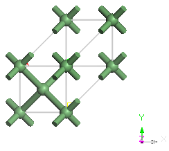
Begin by importing the Ge structure, which is included in the structure library provided with Materials Studio.
Select File | Import... from the menu bar to open the Import Document dialog. Navigate to Structures/metals/pure-metals and select Ge.xsd.
2. To optimize the structure of the germanium cell
It is often possible to get significant speedup by converting the structure to a primitive cell.
Select Build | Symmetry | Primitive Cell from the menu bar.
The primitive germanium cell is displayed.
Now optimize the geometry of the Ge structure using CASTEP.
Click the CASTEP button
 on the Modules toolbar and select
Calculation or choose Modules | CASTEP | Calculation from the menu bar.
on the Modules toolbar and select
Calculation or choose Modules | CASTEP | Calculation from the menu bar.
This opens the CASTEP Calculation dialog.
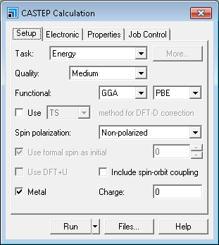
CASTEP Calculation dialog, Setup tab
The default values for geometry optimization do not include optimization of the cell.
On the Setup tab change the Task from Energy to
Geometry Optimization and the Functional to LDA.
Uncheck the Metal checkbox as Ge is a semiconductor.
Change Quality to
Ultra-fine, which is a recommended setting for calculating vibrational properties of materials.
Click the More... button to open the CASTEP Geometry Optimization dialog, select Full from the Cell optimization dropdown list and close the dialog.
Select the Electronic tab of the CASTEP Calculation dialog and set Pseudopotentials to
Norm conserving (linear response calculations of phonon properties are available only for norm-conserving potentials).
On the Job Control tab select the location for the job to run in the Gateway location dropdown list, and set the Runtime optimization to Speed.
Click the Run button to start the job.
The job is submitted and starts to run. It should take a few minutes, depending on the speed of your computer.
The results are placed in a new folder called Ge CASTEP GeomOpt.
3. To calculate phonon dispersion and phonon density of states (DOS)
DFPT gives an opportunity to accurately calculate phonon frequencies at any given point in reciprocal space. However, a calculation for each q-point can be expensive. An alternative approach may be used for calculations that require phonon frequencies for large numbers of q-points, for example, for phonon DOS and thermodynamic properties. This alternative scheme takes advantage of the relatively short range of effective ion-ion interactions in crystals. Interpolation can be used to reduce computation time without loss of accuracy. The accurate DFPT calculations are performed only at a small number of q-vectors, and then a cheap interpolation procedure is used to obtain frequencies at other q-points of interest. One advantage of using an interpolation scheme instead of the exact calculation is that thermodynamic properties at low temperatures depend strongly on the number of points in the phonon DOS grid. Using the interpolation approach, this number can be increased at no computational cost.
In order to calculate the phonon dispersion and phonon density of states you must perform a single point energy calculation, after selecting the appropriate properties from the Properties tab on the CASTEP Calculation dialog.
Ensure that Ge.xsd in the Ge CASTEP GeomOpt folder is the
active document.
On the Setup tab of the CASTEP Calculation dialog set the
Task to Energy.
On the Properties tab choose Phonons and request
Density of states and Dispersion by selecting the Both option.
Click the More... button, to display the CASTEP Phonon Properties Setup dialog.
Ensure the Method is Linear response and the Use
interpolation checkbox is checked. Ensure that q-vector grid spacing for interpolation is
0.05 1/Å, and the Quality for Dispersion and
Density of states is set to Fine. Close the dialog.
Click the Run button and close the CASTEP Calculation dialog.
The job is submitted and starts to run. This is a more time-consuming job and could take about 10 minutes on a multi-core computer. A new folder, called Ge CASTEP Energy, is created in the Ge CASTEP GeomOpt folder.
When the energy calculation is finished two new results files are placed in this folder, Ge_PhonDisp.castep and
Ge_PhonDOS.castep.
4. To display phonon dispersion and density of states
Phonon dispersion curves show how phonon energy depends on the q-vector, along high symmetry directions in the
Brillouin zone. This information can be obtained experimentally from neutron scattering experiments on single crystals.
Such experimental data are available for only a small number of materials, so theoretical dispersion curves are
useful for establishing the validity of a modeling approach to demonstrate the predictive power of ab initio
calculations. In certain circumstances it is possible to measure the density of states (DOS) rather than the phonon
dispersion. Furthermore, the electron-phonon interaction function, which is directly related to the phonon DOS can be
measured directly in the tunneling experiments. It is therefore important to be able to calculate phonon DOS from first
principles. Materials Studio can produce phonon dispersion and DOS charts from any .phonon CASTEP output file. These
files are hidden in the Project Explorer but a .phonon file is generated with every .castep file that has a PhonDisp
or PhonDOS suffix.
When evaluating phonon DOS, use only the results of phonon calculations on the Monkhorst-Pack grid.
Now use the results of the previous calculation to create a phonon dispersion chart.
Select Modules | CASTEP | Analysis from the menu bar to open the CASTEP Analysis dialog. Choose
Phonon dispersion from the list of properties. Ensure that the Results file
selector displays Ge_PhonDisp.castep.
Select cm-1 from the Units dropdown list and Line
from the Graph style dropdown list.
Click the View button.
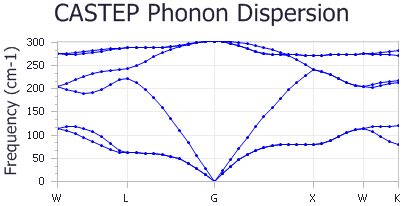
A new chart document, Ge Phonon Dispersion.xcd, is created in the results folder. It should look something like the
chart shown below:
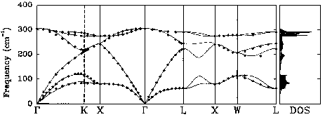
The experimental phonon dispersion is shown below:
The predicted frequencies are available in the Ge_PhonDisp.castep file.
Double-click on Ge_PhonDisp.castep in the Project Explorer. Press CTRL + F and search for Vibrational Frequencies.
The following portion of the results file is displayed:
 ==============================================================================
 +                           Vibrational Frequencies                          +
 +                           -----------------------                          +
 +                                                                            +
 + Performing frequency calculation at  40 wavevectors (q-pts)                +
 + ========================================================================== +
 +                                                                            +
 + -------------------------------------------------------------------------- +
 +  q-pt=    1 (  0.500000  0.250000  0.750000)     0.0487804878              +
 + -------------------------------------------------------------------------- +
 +  Acoustic sum rule correction <   0.002528 cm-1 applied                    +
 +     N      Frequency irrep.                                                +
 +                (cm-1)                                                      +
 +                                                                            +
 +     1     114.828225   a                                                   +
 +     2     114.828225   a                                                   +
 +     3     204.776057   b                                                   +
 +     4     204.776057   b                                                   +
 +     5     274.984105   a                                                   +
 +     6     274.984105   a                                                   +
 + .......................................................................... +
 +        Character table from group theory analysis of eigenvectors          +
 +                           Point Group =  32, Oh                            +
 + .......................................................................... +
 +  Rep  Mul |    E   2   2   m  -4                                           +
 +           | --------------------                                           +
 + a       2 |    2   0   0   0  -1                                           +
 + b       1 |    2   0   0   0   1                                           +
 + -------------------------------------------------------------------------- +
....
The results you obtain may vary slightly from those shown because of minor differences in the structure of the starting model.
The frequencies for every q-point and for every branch (Longitudinal Optical or Acoustical (LO/LA), Transverse Optical or Acoustical (TO/TA)) are given in cm-1, as well as the positions of the q-points, in the reciprocal space. The high symmetry points Γ, L and X are at reciprocal space positions (0 0 0), (0.5 0.5 0.5) and (0.5 0 0.5) respectively.
The predicted and experimental frequencies in cm-1 are:
| Predicted | Experimental | |
|---|---|---|
| ΓTO | 302 | 304 |
| ΓLO | 302 | 304 |
| ΓTA | 0 | 0 |
| ΓLA | 0 | 0 |
| LTA | 62 | 63 |
| LLA | 223 | 222 |
| LTO | 243 | 245 |
| LLO | 288 | 290 |
| XTA | 80 | 80 |
| XLA | 241 | 241 |
| XTO | 272 | 276 |
Overall, the accuracy of the calculation is acceptable. Better agreement with the experimental results may be obtained by running the calculation with a better SCF k-point grid.
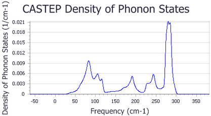
Now create a phonon DOS chart.
On the CASTEP Analysis dialog select Phonon density of states from the list of properties.
Make Ge.xsd the active document and ensure that the Results file selector displays
Ge_PhonDOS.castep.
Set Display DOS to Full. Click the More...
button to open the CASTEP Phonon DOS Analysis Options dialog. Select Interpolation from the
Integration method dropdown list and set the Accuracy level to
Fine. Click the OK button and on the CASTEP Analysis dialog click the
View button to create the DOS chart.
Interpolation scheme was chosen to get the best representation of DOS; an alternative setting, smearing, produces DOS with too few fine details.
A new chart document, Ge Phonon DOS.xcd, is created. It should look something like the chart shown below:
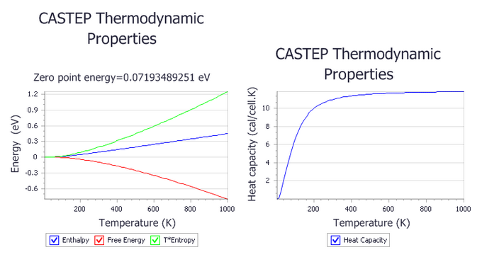
5. To display thermodynamic properties
Phonon calculations in CASTEP can be used to evaluate the temperature dependence of the enthalpy, entropy, free energy, and lattice heat capacity of a crystal in a quasi-harmonic approximation. These results can be compared with experimental data (for example heat capacity measurements) or used to predict phase stability of different structural modifications or phase transitions.
All energy-related properties are plotted on one graph, and the calculated value of the zero-point energy is included. The heat capacity is plotted separately on the right.
The entropy is present as a TS product to allow comparison with the enthalpy.
Now use the results of the phonon calculation to create a thermodynamic properties chart.
On the CASTEP Analysis dialog choose
Thermodynamic properties from the list of properties. Make Ge.xsd the active document and
ensure that the Results file selector displays Ge_PhonDOS.castep.
Check the Plot Debye temperature checkbox and click the View button.
Two new chart documents, Ge Thermodynamic Properties.xcd and Ge Debye Temperature.xcd,
are created in the results folder:
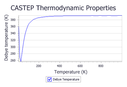
Experimental results without anharmonicity (Flubacher et al., 1959) show that the Debye temperature at the high temperature limit is 395(3) K. The simulated Debye temperature is 392 K, in excellent agreement with the experimental value.
Overall, the experimental plot is qualitatively very similar to the one generated by CASTEP. There is a dip at about 25 K, with the lowest value of Debye temperature of the order of 255 K, exactly as predicted by CASTEP results. The exact shape of the curve at very low temperatures is not accurate with the calculation settings used in this tutorial. A better sampling of low-frequency acoustic modes is required, and this can be achieved by using a finer Monkhorst-Pack grid in the phonon density of states calculation.
6. To display atomic displacement parameters
Atomic displacement parameters, also known as temperature factors, can be estimated from phonon calculations and displayed in the visualizer as ellipsoids.
On the CASTEP Analysis dialog choose
Thermodynamic properties from the list of properties. Make Ge.xsd the active document and
ensure that the Results file selector displays Ge_PhonDOS.castep.
Click Assign temperature factors to structure button.
This action adds information about anisotropic temperature factors to each atom. The values can be examined using Properties Explorer. The value of the B factor produced in this tutorial, 0.545 Å2, is in excellent agreement with experimental reports (between 0.52 and 0.55 Å2).
In order to visualize temperature factors as ellipsoids, open the Temperature Factor tab of the Display Style dialog and click Add. Ellipsoids are added to the display, but they might be obscured by the reciprocal space objects. You can hide reciprocal space objects by clearing the Display reciprocal lattice checkbox on the Reciprocal tab of the Display Style dialog.
This is the end of the tutorial.
References
Flubacher, P.; Leadbetter, A. J.; Morrison, J. A. "The heat capacity of pure silicon and germanium and properties of their vibrational frequency spectra", Phil. Mag., 4, 273-294 (1959).