Predicting the lattice parameters of AlAs from first principles

Purpose: Introduces geometry optimization in CASTEP and the use of the volume visualization tools to display isosurfaces.

Modules: Materials Visualizer, CASTEP

Time: 

Prerequisites: Using the crystal builder

Background

Recent developments in density functional theory (DFT) methods applicable to studies of large periodic systems have become essential in addressing problems in materials design and processing. The DFT tools can be used to guide and lead the design of new materials, allowing researchers to understand the underlying chemistry and physics of processes.

Introduction

This tutorial illustrates how CASTEP can be used to determine the lattice parameters and electronic structure of aluminum arsenide using quantum mechanical methods in Materials Studio. You will learn how to build a crystal structure and set up a CASTEP geometry optimization run, and then analyze the results.

This tutorial covers:

• Getting started
• To build an AlAs crystal structure
• To set up and run the CASTEP calculation
• To analyze the results
• To compare the structure with experimental data
  • Visualizing the charge density
  • Density of states and band structure

In order to ensure that you can follow this tutorial exactly as intended, you should use the Settings Organizer dialog to ensure that all your project settings are set to their BIOVIA default values. See the Creating a project tutorial for instructions on how to restore default project settings.

1. Getting started

Begin by starting Materials Studio and creating a new project.

Open the New Project dialog and enter AlAs_lattice as the project name, click the OK button.

The new project is created with AlAs_lattice listed in the Project Explorer. The next step is to create a document in which to generate the AlAs lattice.

In the Project Explorer, right-click on the root and select New | 3D Atomistic Document from the shortcut menu. Rename the new document AlAs.xsd.

2. To build an AlAs crystal structure

To build a crystal structure, you need to know the space group, lattice parameters, and internal coordinates for the crystal you wish to construct. In the case of AlAs, the space group is F-43m, number 216. There are two atoms in the basis, Al and As with fractional coordinates of (0, 0, 0) and (0.25, 0.25, 0.25), respectively. The lattice parameter is 5.6622 Å.

The first step is to build the lattice.

Choose Build | Crystals | Build Crystal... from the menu bar.

This opens the Build Crystal dialog.

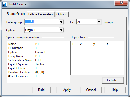
Build Crystal dialog, Space Group tab

Click in the Enter group box and type 216, press TAB.

The Space group information box updates with the information for the F-43m space group.

Select the Lattice Parameters tab. Change the value of a from 10.00 to 5.6622. Press TAB and click the Build button.

An empty 3D lattice is displayed in the 3D Viewer, now you can add the atoms.

Select Build | Add Atoms from the menu bar.

This opens the Add Atoms dialog.

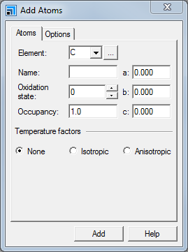
Add Atoms dialog, Atoms tab

Using this dialog, you can add atoms at specific positions.

On the Add Atoms dialog, select the Options tab and ensure that the Coordinate system is set to Fractional. Select the Atoms tab, in the Element text box type Al. Click the Add button.

The aluminum atoms are added to the structure.

In the Element text box, type As. Enter 0.25 into the a, b, and c text boxes. Click the Add button and close the dialog.

The atoms are added and the symmetry operators are used to build the remaining atoms in the crystal structure. The atoms are also displayed in neighboring unit cells to illustrate the bond topology of the AlAs structure. You can remove these by rebuilding the crystal.

Choose Build | Crystals | Rebuild Crystal... from the menu bar to open the Rebuild Crystal dialog. Click the Rebuild button.

The extraneous atoms are removed and the crystal structure is displayed. You can change the display style to ball and stick.

Right-click in the structure document and select Display Style from the shortcut menu. On the Atom tab, select the Ball and stick option and close the dialog.

The crystal structure in the 3D Viewer is the conventional unit cell, which shows the cubic symmetry of the lattice. CASTEP uses the full symmetry of the lattice if any exists. So the primitive lattice, containing 2 atoms per unit cell, can be used, as opposed to the conventional cell, which contains 8 atoms. The charge density, bond distances, and total energy per atom will all be the same no matter how the unit cell is defined, so by using fewer atoms in the unit cell the computation time will be decreased.

When a spin-polarized calculation is performed on a magnetic system care should be taken if the charge density spin wave has a period which is a multiple of the primitive unit cell.

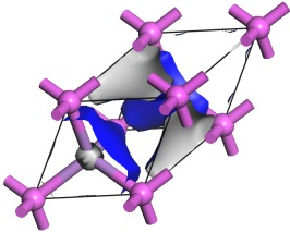
Choose Build | Symmetry | Primitive Cell from the menu bar.

The 3D Viewer displays the primitive cell.

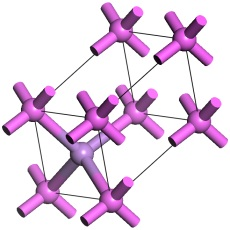
The primitive cell of AlAs

3. To set up and run the CASTEP calculation

Click the CASTEP button on the Modules toolbar and select Calculation or choose Modules | CASTEP | Calculation from the menu bar

This opens the CASTEP Calculation dialog.

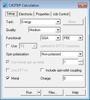
CASTEP Calculation dialog, Setup tab

You are going to optimize the geometry of the structure.

Change the Task to Geometry Optimization and the Quality to Fine.

The default setting for optimization is to optimize only the atomic coordinates. However, in this case, you want to optimize the lattice since the atomic coordinates in AlAs structure are fixed by symmetry.

Click the More... button for the Task to open the CASTEP Geometry Optimization dialog. Select Full from the Cell optimization dropdown list and close the dialog.

When you change the quality, the other parameters change to reflect this.

Select the Properties tab.

You can specify which properties you want to calculate from the Properties tab.

Check the Band structure and Density of states checkboxes.

With the Band structure option selected, click the More... button to open the CASTEP Band Structure Options dialog. Click the Path... button to open the Brillouin Zone Path dialog. Click the Create button and close both dialogs.

The reciprocal lattice and Brillouin zone paths and axes are displayed in the 3D viewer.

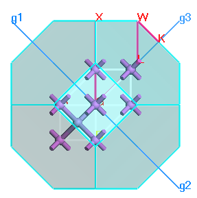
AlAs reciprocal lattice and Brillouin zone paths

You can also specify job control options such as live updates.

Select the Job Control tab. Click the More... button to open the CASTEP Job Control Options dialog. Change the Update interval to 5.0 s and close the dialog.

If you are running the calculation on a remote server, you can specify this from the Job Control tab.

Click the Run button and close the CASTEP Calculation dialog.

After a few seconds, a new folder is displayed in the Project Explorer and this will contain all the results from the calculation. The Job Explorer is displayed, which contains information about the status of the job.

The Job Explorer displays the status of any currently active jobs that are associated with this project. It shows useful information such as the server and job identification number. You can also use this explorer to stop the job if you need to.

As the job progresses, four documents open which relay information on the job status. These documents include the crystal structure, showing updates of the model during optimization, a status document to relay information about the job setup parameters and run information, and charts of the total energy, and convergence in energy, forces, stress, and displacement as a function of the iteration number.

When the job finishes, the files are transferred back to the client and this can take some time due to the size of certain files.

4. To analyze the results

When the results documents are transferred, you should have several documents, among them:

• AlAs.xsd - the final optimized structure
• AlAs.xtd - a trajectory file containing the structure after each optimization step
• AlAs.castep - an output text document containing the optimization information
• AlAs.param - input information for the simulation

For each of the properties calculated, there are also .param and .castep documents.

In the AlAs structure, the forces are zero by symmetry, but the stresses depend on the lattice parameters. CASTEP thus attempts to minimize the total energy by finding the structure that corresponds to the zero stress. Therefore, to ensure that the calculation has completed properly, it is important to check that the stresses have converged.

Make AlAs.castep the active document and select Edit | Find... from the menu bar to open the Find dialog. Enter completed successfully in the text box and click the Find Next button. Scroll a few lines up.

You will see a table containing two rows, and the last column in each row should say Yes. This indicates that the calculation has succeeded.

5. To compare the structure with experimental data

You know that the lattice length should be 5.6622 Å from when you initially created the cell. You can compare your minimized lattice length with that of the initial experimental length. The experimental lattice length is based on a conventional cell and not a primitive one, so you should convert your cell.

Make the optimized AlAs.xsd the active document and select Build | Symmetry | Conventional Cell from the menu bar.

The conventional cell is displayed. There are several ways to view the lattice lengths, but the easiest is to open the Lattice Parameters dialog.

Right-click in the 3D Viewer and select Lattice Parameters from the shortcut menu.

The lattice vector should be approximately 5.731 Å, giving an error of about 1%. This is within the 1-2% typical error that is expected for pseudopotential plane-wave methods in comparison with experimental results. An over-estimation of the lattice parameters is typical of the GGA functional, use of LDA functionals may result in under-estimation.

Before continuing, you should save the project and close all the windows.

Choose File | Save Project on the menu bar, then Window | Close All.

The charge density can be visualized using the CASTEP Analysis tool.

Click the CASTEP button on the Modules toolbar and select Analysis or choose Modules | CASTEP | Analysis from the menu bar to display the CASTEP Analysis dialog.

Choose the Electron density option.

A message is displayed reporting that no results file is available, so you need to specify a results file.

In the Project Explorer, double-click on AlAs.castep.

This will associate the results document with the analysis dialog but you also need to designate a 3D Atomistic document in which to display the isosurface.

In the Project Explorer, double-click on the optimized AlAs.xsd. Choose Build | Symmetry | Primitive Cell from the menu bar.

The Import button on the CASTEP Analysis dialog is now active.

Click the Import button.

The isosurface is overlaid onto the structure.

Electron density isosurface of AlAs

You can change the isosurface settings using the Display Style dialog.

Open the Display Style dialog and select the Isosurface tab.

Display Style dialog, Isosurface tab

You can change various settings here.

In the Isovalue text box, type 0.1 and press TAB.

Note how the isosurface changes.

Move the Transparency slider bar to the right.

As you move the Transparency slider bar, the surface becomes more transparent.

Hold down the right mouse button and move the mouse to rotate the model.

As the model rotates, the isosurface reverts to a dot display to increase the speed of rotation. If you have a fast machine, you can disable this feature by unchecking the Fast render on move checkbox on the Graphics tab of the Display Options dialog.

You can toggle display of the isosurface at any time by checking or unchecking the Visible checkbox on the Isosurface tab of the Display Style dialog.

You can display the Brillouin zone path for the reciprocal lattice, see the Brillouin zone theory topic for further information.

Select Tools | Brillouin Zone Path from the menu bar to open the Brillouin Zone Path dialog. Click the Create button and close the dialog.

The Brillouin zone and k-paths display can be manipulated using the Display Style dialog.

Select the Reciprocal tab and move the Transparency slider all the way to the right. Set the Scale to 33 and change the Path Line width to 5.00. Close the dialog.

Rotate the structure to view the high-symmetry points and the standard Brillouin zone path for this lattice type.

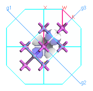
Brillouin zone paths and isosurface of AlAs

The CASTEP Analysis tool can be used to display density of states, DOS, and band structure information.

Band structure charts show the dependence of electronic energies on k-vector along high symmetry directions in the Brillouin zone. These charts provide a useful tool for qualitative analysis of the electronic structure of the material - for example, it is easy to identify narrow bands of d and f states as opposed to nearly free electron-like bands that correspond to s and p electrons.

DOS and PDOS charts give a quick qualitative picture of the electronic structure of the material, and sometimes they can be directly related to experimental spectroscopic results.

The main CASTEP output file, AlAs.castep, contains limited band structure and DOS information, but more detailed information is contained in the AlAs_BandStr.castep and AlAs_DOS.castep documents, respectively.

On the CASTEP Analysis dialog select the Band structure option.

From this dialog, you can choose to display both the band structure and density of states information on the same chart document and control the DOS chart quality.

You can also display them in separate chart documents by analyzing the band structure and density of states separately.

Check the Show DOS checkbox and click the More... button to open the CASTEP DOS Analysis Options dialog. Set the Integration method to Interpolation and the Accuracy level to Fine. Click the OK button.

On the CASTEP Analysis dialog, click the View button.

A chart document is generated containing the band structure and density of states charts.

You can export any chart document as a comma-separated variable file which can then be read in any spreadsheet package, for example, Excel.

You can also use CASTEP to calculate many other properties, such as reflectivity and dielectric functions.

This is the end of the tutorial.