Calculating elastic constants for BN
Purpose: Illustrates the use of CASTEP to calculate elastic constants.
Modules: Materials Visualizer, CASTEP
Time: 
Prerequisites: Predicting the lattice parameters of AlAs from first principles
Background
Recent developments in density functional theory (DFT) methods applicable to studies of large periodic systems have become essential in addressing problems in materials design and processing. The DFT tools can be used to guide and lead the design of new materials, allowing researchers to understand the underlying chemistry and physics of processes.
Introduction
In this tutorial, you will learn how to use CASTEP to calculate elastic constants and other mechanical properties. In the first part you will optimize the structure of cubic BN and then you will calculate its elastic constants.
This tutorial covers:
- Getting started
- To optimize the structure of cubic BN
- To calculate the elastic constants of BN
- Description of the elastic constants file
In order to ensure that you can follow this tutorial exactly as intended, you should use the Settings Organizer dialog to ensure that all your project settings are set to their BIOVIA default values. See the Creating a project tutorial for instructions on how to restore default project settings.
Begin by starting Materials Studio and creating a new project.
Open the New Project dialog and enter BN_elastic as the project name, click the OK button.
The new project is created with BN_elastic listed in the Project Explorer. The next step is to import the BN structure.
Select File | Import... from the menu bar to open the Import Document dialog. Navigate to the folder Structures/semiconductors/ and select BN.xsd. Click the Open button.
The crystal structure of BN is displayed.
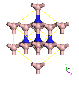
Structure of BN cubic
This is the conventional representation of the BN structure. In order to reduce the computation time, you should convert to the primitive representation.
Select Build | Symmetry | Primitive Cell from the menu bar.
2. To optimize the structure of BN cubic
It is not necessary to perform geometry optimization before calculating elastic constants, so you can generate Cij data for experimentally observed structures. However, more consistent results are obtained if you perform full geometry optimization, including cell optimization, and then calculate the elastic constants for the structure corresponding to the theoretical ground state.
The accuracy of the elastic constants, especially of the shear constants, depends strongly on the quality of the SCF calculation and, in particular, on the quality of the Brillouin zone sampling and the degree of convergence of wavefunctions. Therefore, you should use the Fine setting for SCF tolerance and k-point sampling and a Fine derived FFT grid.
Now you will set up the geometry optimization.
Click the CASTEP button  on the
Modules toolbar and select Calculation from the dropdown list or choose
Modules | CASTEP | Calculation from the menu bar.
on the
Modules toolbar and select Calculation from the dropdown list or choose
Modules | CASTEP | Calculation from the menu bar.
This opens the CASTEP Calculation dialog.
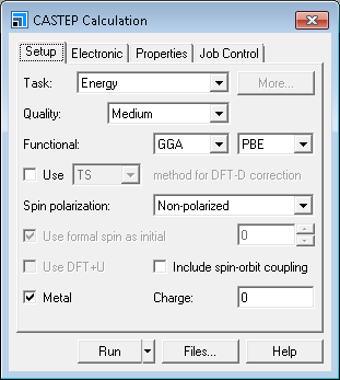
CASTEP Calculation dialog, Setup tab
On the Setup tab, set the Task to Geometry
Optimization, the Quality to Fine, and the
Functional to GGA and PBESOL.
Click the More... button to open the CASTEP Geometry Optimization dialog. Select Full from the Cell optimization dropdown list and close the dialog.
Choose the Job Control tab on the CASTEP Calculation dialog and select the Gateway on which
you wish to run the CASTEP job.
Click the Run button.
After optimization, the structure should have cell parameters of about a = b = c = 2.553 Å which corresponds to 3.610 Å lattice parameter for the conventional unit cell (experimental value is 3.615 Å).
Right-click in the 3D Viewer and select Lattice Parameters from the shortcut menu.
The lattice parameters are shown. Now you can go on to calculate the elastic constants of the optimized structure.
3. To calculate the elastic constants of BN
Select the Setup tab on the CASTEP Calculation dialog. Select Elastic Constants from the Task dropdown list and click the More... button.
This opens the CASTEP Elastic Constants dialog.
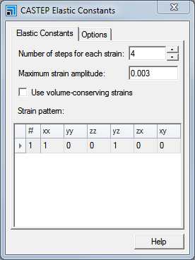
CASTEP Elastic Constants dialog, Elastic Constants tab
Increase the Number of steps for each strain from 4 to 6 and close the dialog. Ensure that BN CASTEP GeomOpt/BN.xsd is the active document and click the Run button on the CASTEP Calculation dialog.
If BN CASTEP GeomOpt/BN.xsd is made active before the CASTEP Elastic
Constants dialog is opened, the Strain pattern grid on this dialog will contain values.
CASTEP results for the Elastic Constants task are returned as a set of .castep output files. Each of them represents
a geometry optimization run with a fixed cell, for a given strain pattern and strain amplitude. The naming convention for these files is:
seedname_cij__m__n
where m is the current strain pattern and n is the current strain amplitude for the given pattern.
CASTEP can use these results to analyze the calculated stress tensors for each of these runs and generate a file with information about elastic properties.
Click the CASTEP button on the
Modules toolbar and select Analysis from the dropdown list or choose
Modules | CASTEP | Analysis from the menu bar.
Select the Elastic constants option. The results file from the Elastic Constants job for BN should
be displayed automatically in the Results file selector. Click the Calculate button.
A new text document, BN Elastic Constants.txt, is created in the results folder.
The information in this document includes a summary of the input strains and calculated stresses, results of linear fitting for each strain pattern (including quality of the fit), the correspondence between calculated stresses and elastic constants for a given symmetry, a table of elastic constants (Cij) and elastic compliances (Sij). The derived properties, such as bulk modulus and its inverse, compressibility, Young modulus, and Poisson ratios for three directions, and the Lamé constants that are needed for modeling the material as an isotropic medium, are also reported in this document.
4. Description of the elastic constants file
The results you obtain may vary slightly from those shown because of minor differences in the structure of the starting model.
Only one strain pattern is required for this lattice type. There is a summary of calculated stresses as extracted from the
respective .castep files:
  ===============================================
  Elastic constants from Materials Studio: CASTEP
  ===============================================

         Summary of the calculated stresses
         **********************************

  Strain pattern:      1
  ======================

  Current amplitude: 1
  Transformed stress tensor (GPa) :
       -8.185512       -0.000000       -0.000000
       -0.000000      -10.013060        1.374720
       -0.000000        1.374720      -10.013060

  Current amplitude: 2
  Transformed stress tensor (GPa) :
       -9.116397       -0.000000       -0.000000
       -0.000000      -10.216359        0.838757
       -0.000000        0.838757      -10.216359

  Current amplitude: 3
  Transformed stress tensor (GPa) :
      -10.048265       -0.000000       -0.000000
       -0.000000      -10.416350        0.292454
       -0.000000        0.292454      -10.416350

  Current amplitude: 4
  Transformed stress tensor (GPa) :
      -10.989498       -0.000000       -0.000000
       -0.000000      -10.613108       -0.258026
       -0.000000       -0.258026      -10.613108

  Current amplitude: 5
  Transformed stress tensor (GPa) :
      -11.916355       -0.000000       -0.000000
       -0.000000      -10.807650       -0.799337
       -0.000000       -0.799337      -10.807650

  Current amplitude: 6
  Transformed stress tensor (GPa) :
      -12.830064       -0.000000       -0.000000
       -0.000000      -10.994485       -1.332785
       -0.000000       -1.332785      -10.994485
All the information about the connection between components of the stress, strain, and elastic constants tensors is provided. At this stage, each elastic constant is represented by a single compact index rather than by a pair of ij indices. The correspondence between the compact notation and the conventional indexing is provided later in the file:
Stress corresponds to elastic coefficients (compact notation):
   1  7  7  4  0  0

 as induced by the strain components:
   1  1  1  4  0  0
A linear fit of the stress-strain relationship for each component of the stress is given in the following format:
     Stress    Cij       value of          value of
     index    index       stress            strain
       1        1        -8.185512         -0.003000
       1        1        -9.116397         -0.001800
       1        1       -10.048265         -0.000600
       1        1       -10.989498          0.000600
       1        1       -11.916355          0.001800
       1        1       -12.830064          0.003000
C (gradient)     :     775.330167
Error on C       :       1.606541
Correlation coeff:       0.999991
Stress intercept :     -10.514348

       2        7       -10.013060         -0.003000
       2        7       -10.216359         -0.001800
       2        7       -10.416350         -0.000600
       2        7       -10.613108          0.000600
       2        7       -10.807650          0.001800
       2        7       -10.994485          0.003000
C (gradient)     :     163.756095
Error on C       :       1.145946
Correlation coeff:       0.999902
Stress intercept :     -10.510169

       3        7       -10.013060         -0.003000
       3        7       -10.216359         -0.001800
       3        7       -10.416350         -0.000600
       3        7       -10.613108          0.000600
       3        7       -10.807650          0.001800
       3        7       -10.994485          0.003000
C (gradient)     :     163.756095
Error on C       :       1.145946
Correlation coeff:       0.999902
Stress intercept :     -10.510169

       4        4         1.374720         -0.003000
       4        4         0.838757         -0.001800
       4        4         0.292454         -0.000600
       4        4        -0.258026          0.000600
       4        4        -0.799337          0.001800
       4        4        -1.332785          0.003000
C (gradient)     :     452.435405
Error on C       :       1.053660
Correlation coeff:       0.999989
Stress intercept :       0.019297
The gradient provides the value of the elastic constant (or a linear combination of elastic constants); the quality of the fit, indicated by the correlation coefficient, provides the statistical uncertainty of that value. The stress intercept value is not used in further analysis, it is simply an indication of how far the converged ground state was from the initial structure.
The results for all the strain patterns are then summarized:
  ============================
  Summary of elastic constants
  ============================

 id  i  j       Cij (GPa)
 1   1  1     775.33017 +/-   1.607
 4   4  4     452.43540 +/-   1.054
 7   1  2     163.75610 +/-   0.810
The errors are only provided when more than two values for the strain amplitude are used, since there is no statistical uncertainty associated with fitting a straight line to only two points.
Elastic constants are then presented in a conventional 6 × 6 tensor form, followed by a similar 6 x 6 representation of the compliances:
      =====================================
      Elastic Stiffness Constants Cij (GPa)
      =====================================

   775.33017   163.75610   163.75610     0.00000     0.00000     0.00000
   163.75610   775.33017   163.75610     0.00000     0.00000     0.00000
   163.75610   163.75610   775.33017     0.00000     0.00000     0.00000
     0.00000     0.00000     0.00000   452.43540     0.00000     0.00000
     0.00000     0.00000     0.00000     0.00000   452.43540     0.00000
     0.00000     0.00000     0.00000     0.00000     0.00000   452.43540

      ========================================
      Elastic Compliance Constants Sij (1/GPa)
      ========================================

   0.0013923  -0.0002428  -0.0002428   0.0000000   0.0000000   0.0000000
  -0.0002428   0.0013923  -0.0002428   0.0000000   0.0000000   0.0000000
  -0.0002428  -0.0002428   0.0013923   0.0000000   0.0000000   0.0000000
   0.0000000   0.0000000   0.0000000   0.0022103   0.0000000   0.0000000
   0.0000000   0.0000000   0.0000000   0.0000000   0.0022103   0.0000000
   0.0000000   0.0000000   0.0000000   0.0000000   0.0000000   0.0022103
The final part of the file contains the derived properties:
Bulk modulus              =   367.61412 +/-  0.761 (GPa)

Compressibility           =     0.00272 (1/GPa)

Elastic Debye temperature =  1888.24550 K
Averaged sound velocity   = 11448.15958 (m/s)

  Axis   Young Modulus        Poisson Ratios
         (GPa)
   X      718.21921       Exy=  0.1744 Exz=  0.1744
   Y      718.21921       Eyx=  0.1744 Eyz=  0.1744
   Z      718.21921       Ezx=  0.1744 Ezy=  0.1744

      ====================================================
      Elastic constants for polycrystalline material (GPa)
      ====================================================

                                      Voigt       Reuss        Hill
Bulk modulus                   :     367.61412   367.61412   367.61412
Shear modulus (Lame Mu)        :     393.77606   379.61381   386.69494
Lame lambda                    :     105.09675   114.53824   109.81750
Young modulus                  :     870.50830   847.21734   858.91818
Poisson ratio                  :       0.10533     0.11589     0.11059
Hardness (Tian 2012)           :      68.41824    63.94740    66.16553
Fracture toughness  (MPa m^0.5):       5.11167     5.01890     5.06550

Universal anisotropy index:       0.18653
The values reported above are roughly within 10% of experimentally measured values (B=396 GPa, C11=820 GPa, C12=190 GPa, C44=457 GPa) which is typical for DFT calculations.
Calculated elastic properties of crystals are significantly more sensitive to the accuracy of the electronic structure calculation than, for example, calculated lattice parameters and atomic coordinates. It is always necessary to check the convergence of the calculated properties with respect to the following parameters:
- density of k-points (most important)
- energy cutoff
- augmentation density scaling factor - in the case of ultrasoft pseudopotentials, either generated on the fly or tabulated ones
An additional consideration in elastic properties calculations is the choice of exchange-correlation functional. Modern functionals that are designed to reproduce solid state properties more accurately than traditional LDA or PBE functionals are PBESOL and Wu-Cohen; these are recommended for calculating elastic coefficients of solids.
This is the end of the tutorial.