Assigning the ¹⁷O NMR spectrum of L-alanine

Purpose: Introduces the capabilities of NMR CASTEP and the use of the visualization tools for displaying isotropic shielding values.

Modules: Materials Visualizer, CASTEP, NMR CASTEP

Time:  

Prerequisites: Predicting the lattice parameters of AlAs from first principles

Background

NMR CASTEP predicts the NMR chemical shielding of molecules and solid-state materials from first principles. Based on density functional theory (DFT), NMR CASTEP provides a way to predict key magnetic resonance properties, NMR chemical shielding and electric field gradient (EFG) tensors, with unprecedented accuracy. The method can be applied to compute the NMR shifts of molecules, solids, interfaces, and surfaces for a wide range of materials classes including organic molecules, ceramics and semiconductors. First-principles calculations allow researchers to investigate the nature and origin of the magnetic resonance properties of a system without the need for any empirical parameters.

NMR is often used as an analytical tool to aid in structure prediction. The relative complexity of solid-state structures makes this a challenging task. Often, even though the general features of the crystal structure are understood, a detailed analysis of the geometry proves elusive. Using NMR CASTEP it is possible to simulate the NMR spectrum for a series of related structures until a match is discovered between the computed and experimental results. In this way, theory complements experiment, with both contributing to the determination of the structure.

NMR in CASTEP is part of the separately licensed module NMR CASTEP. NMR calculations can only be performed if you have purchased this module.

Introduction

In this tutorial, you will use NMR CASTEP to assign the observed ¹⁷O chemical shifts to the two unique atoms in crystalline L-alanine. You will learn how to run an NMR CASTEP calculation, display the results in the Materials Visualizer, and to interpret the results.

L-Alanine is one of the smaller amino acids. The unit cell contains 4 molecules for a total of 48 atoms. There are 2 distinct oxygen sites. This tutorial will use the computed NMR chemical isotropic shielding values to tell them apart. Experiment can also distinguish between the two oxygens, but only with a very sophisticated solid-state NMR apparatus.

This tutorial covers:

• Getting started
• To run an NMR CASTEP calculation
• To analyze the results
• To compare the results with experimental data

In order to ensure that you can follow this tutorial exactly as intended, you should use the Settings Organizer dialog to ensure that all your project settings are set to their BIOVIA default values. See the Creating a project tutorial for instructions on how to restore default project settings.

1. Getting started

Begin by starting Materials Studio and creating a new project.

Open the New Project dialog and enter NMR_alanine as the project name, click the OK button.

The new project is created with NMR_alanine listed in the Project Explorer. The next step is to import the structure.

Select File | Import... from the menu bar to open the Import Document dialog. Navigate to Examples\Documents\3D Model\ and select the l_alanine.xsd file, click the Open button.

The l_alanine document is displayed.

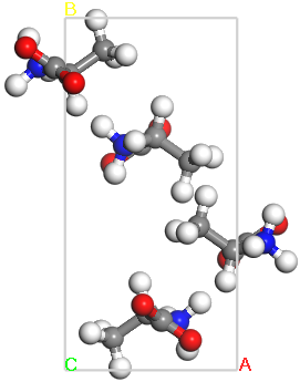
Crystal structure of L-alanine

2. To run an NMR CASTEP calculation

Begin by opening the crystal structure for L-alanine. This is a neutron diffraction crystal structure (Lehmann et al., 1972). You could also build this crystal structure from scratch and optimize it with CASTEP. Using experimental crystal structures, however, yields results comparable with the DFT-optimized geometry and saves computation time.

Click the CASTEP button on the Modules toolbar and choose Calculation or select Modules | CASTEP | Calculation from the menu bar.

This opens the CASTEP Calculation dialog.

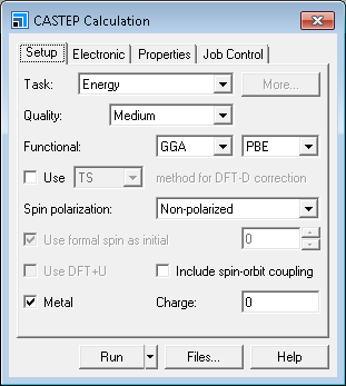
CASTEP Calculation dialog, Setup tab

You are going to run an energy calculation on the structure and request a calculation of the NMR chemical shielding tensor.

Ensure that the Task is set to Energy and the Functional is GGA PBE. Change the Quality to Ultra-fine. Uncheck the Metal checkbox (chemical shielding cannot be calculated for metallic systems).

As a rule, the computed NMR results are sensitive to the Quality of the calculation. In order to obtain results that are comparable with experiment, you should use the Ultra-fine Quality setting. These calculations will take longer than Fine or Medium calculations, but the results are considerably more reliable.

On the Electronic tab select OTFG ultrasoft from the Pseudopotentials dropdown list.

On the fly (OTFG) pseudopotentials are required to compute the magnetic shielding properties. If you choose a different type of pseudopotential, the NMR calculation cannot be performed.

Now specify the properties you want to calculate from the Properties tab.

On the Properties tab check the NMR checkbox and ensure that the Shielding and EFG checkboxes are checked.

This will compute both the NMR chemical shielding and the value of the electric field gradient at the nuclei. If you are running the calculation on a remote server, you can specify the server using the Job Control tab.

On the Job Control tab choose an appropriate server from the Gateway dropdown list.

Click the Run button and close the dialog.

Depending on the speed of the computer you are using the NMR calculation will take a few minutes to complete. Alternatively, rather than running the calculation yourself, you can open the pre-computed results in the Examples folder as described below.

While the calculation is running several things will happen in the Materials Studio interface. After a few seconds, a new folder is displayed in the Project Explorer and this will contain all the results when the calculation is complete. The Job Explorer is displayed, which contains information about the status of the job. The Job Explorer displays the status of any currently active jobs that are associated with this project. It shows useful information such as the server and job identification number. You can also use this explorer to stop the job if you need to.

As the job progresses, four documents open which relay information on the job status. These documents include the crystal structure, a status document to relay information about the job setup parameters and run information, and charts of the total energy and its convergence as a function of the iteration number.

When the job finishes, the files are transferred back to the client and this can take some time due to the size of certain files.

3. To analyze the results

When the results are transferred, you should have several documents, among them:

• l_alanine.xsd - the crystal structure
• l_alanine.castep - an output file from the CASTEP energy calculation
• l_alanine_NMR.castep - an output file from the NMR CASTEP calculation
• l_alanine.param - input information
• l_alanine.castep_bin and l_alanine_NMR.castep_bin - binary files containing a summary of the results. Although not visible in the Explorer, these hidden files are required for the analysis

If you chose to run the NMR calculation, you should find these files in folder called l_alanine CASTEP Energy once the calculation completes.

If you decide not to wait for the job to finish, you can access a pre-computed version of these files as follows.

Use the Windows File Explorer to navigate to the \share\Examples\Projects\CASTEP directory, from the top level of your Materials Studio installation. Double-click on the file l_alanine.stp.

For Windows users who are not administrators, you should copy the l_alanine.stp project and associated l_alanine Files folder to a location where you have write permissions. Then open the new copy of the l_alanine.stp project.

Whether you choose to wait for the long calculation to finish or you decide to open the pre-computed results, the tutorial is the same from this point. If you ran the l_alanine calculations using the Medium Quality setting to save time, the steps are still the same, but your numerical results will differ from the ones discussed here. First, examine the data in the NMR output file.

In the Project Explorer, open l_alanine CASTEP Energy/l_alanine_NMR.castep and locate the line that reads Chemical Shielding and Electric Field Gradient Tensors.

This is located about 100 lines up from the end of the file. The output data will look something like this (for clarity, the results for H, C, and N have been removed):

  ========================================================================
  |           Chemical Shielding and Electric Field Gradient Tensors     |
  |----------------------------------------------------------------------|
  |     Nucleus                Shielding tensor             EFG Tensor   |
  |  Species       Ion    Iso(ppm)   Aniso(ppm)  Asym    Cq(MHz)    Eta  |
  |    O           1      -27.61     419.12      0.49   8.304E+00   0.26 |
  |    O           2       -9.52     307.31      0.66   6.773E+00   0.65 |
  |    O           3      -27.61     419.12      0.49   8.304E+00   0.26 |
  |    O           4       -9.52     307.31      0.66   6.773E+00   0.65 |
  |    O           5      -27.61     419.12      0.49   8.304E+00   0.26 |
  |    O           6       -9.52     307.31      0.66   6.773E+00   0.65 |
  |    O           7      -27.61     419.12      0.49   8.304E+00   0.26 |
  |    O           8       -9.52     307.31      0.66   6.773E+00   0.65 |
  ========================================================================

The results you obtain may vary slightly from those shown because of minor differences in the structure of the starting model.

The magnetic shielding data are displayed for each element that used an OTFG pseudopotential. In the case of L-alanine, this includes the elements, H, C, N, and O. In this tutorial, you will focus on the ¹⁷O results.

The first column of the results simply indicates the element symbol. The second column, called Ion, is the relative order of a particular atom in the input file. The subsequent columns are defined as follows:

• Iso (ppm) - the isotropic chemical shielding in ppm. This is defined as σ_iso = (σ_xx + σ_yy + σ_zz)/3, where σ refers to the chemical shielding tensor in the principal axis frame, that is after diagonalization. This is an absolute value of the isotropic chemical shielding, not relative to a standard.
• Aniso (ppm) - the anisotropy defined as Δ = σ_zz - σ_iso.
• Asym - the asymmetry parameter defined as η = (σ_xx - σ_yy)/Δ.
• Cq (MHz) - the quadrupolar coupling constant, C_Q = eQV_zz/h, where V_zz is the largest component of the diagonalized EFG tensor, Q is the nuclear quadrupole moment, and h is the Planck constant.
• Eta - the quadrupolar asymmetry parameter, η_Q = (V_xx - V_yy)/V_zz.

Scroll down to the results for oxygen. Notice that although there are 8 individual oxygen atoms in the unit cell, there are only 2 distinct results. This is because there are only 2 symmetry-unique oxygen atoms in the cell. Now you will use the Materials Visualizer and the experimental data to determine which NMR signal corresponds to which atom.

Open l_alanine CASTEP Energy/l_alanine.xsd.

Click the CASTEP button on the Modules toolbar, then choose Analysis or select Modules | CASTEP | Analysis from the menu bar to open the CASTEP Analysis dialog.

Choose the NMR option and click the Assign isotropic chemical shielding to structure button.

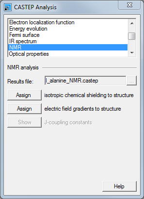
CASTEP Analysis dialog, NMR selection

The isotropic chemical shielding values have been loaded into the structure. Now you will display the shielding values for the oxygen atoms.

Hold down ALT and double-click on any of the oxygen atoms.

This selects all the oxygen atoms in the system.

Right-click in l_alanine.xsd and select Label from the shortcut menu to open the Label dialog. From the Properties select NMRShielding and click the Apply button.

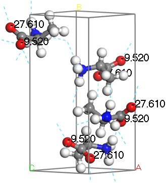
The NMR isotropic shielding values are displayed for the oxygen atoms.

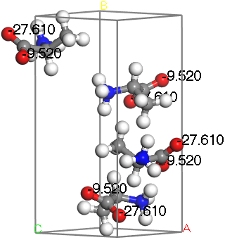
L-Alanine with ¹⁷O isotropic chemical shielding displayed

You can use a similar process to import the electric field gradient data. Atoms can be labeled using either the quadrupolar coupling or the asymmetry parameter.

4. To compare the structure with experimental data

The experimental results for the ¹⁷O magnetic resonance data may be found in Pike et al., (2004). In general, the EFG values and asymmetry parameters can be compared directly with experiment. The isotropic chemical shifts require some analysis because the program reports absolute chemical shielding whereas most experimentalists are concerned with shifts relative to a known standard. This difference can be dealt with in two ways:

1. In most cases, such as in this example, the primary interest is in comparative shifts, which shift is lowest and which is highest, so there is no need to convert the shielding to the same relative standard used by the experiment. The relative positions are all that is needed in order to assign the shifts to atoms unambiguously. This is easy to do because the relative positions of the peaks do not change when shifted with respect to a standard.
2. When dealing with several related systems, it is necessary to determine a value empirically such that you can convert the shielding to a relative shift. Rather than calculate the chemical shielding of the reference compound explicitly, the reference is obtained by comparing it to a system that is experimentally well-characterized and is similar to the systems being investigated. For example, Yates et al. (2004) investigated ¹⁷O shifts for glutamic acid polymorphs. The reference that was chosen was the one which provided the best match between computed and observed values for D-glutamic acid-HCl. The same value was applied to all of the polymorphs.

So, why not compute the value of the standard? Typical standards are liquids like water and tetramethylsilane (TMS). A simple calculation on an isolated molecule is quite easy to do, but yields a result very different from the experimental value. On the other hand, computing a value for the liquid state is a complex task, involving the creation of an accurate model of the liquid and subsequent evaluation of the NMR chemical shielding averaged over time and molecular orientation. The results obtained by comparing to one known experimental system provides a more rapid approach, and in addition, provides an immediate coherence check on the results.

The table below summarizes the computed and observed results.

Quantity	Theory	Experiment
σiso O1 (ppm)	-27.61
δiso O1 (ppm)		284
σiso O2 (ppm)	-9.52
δiso O2 (ppm)		260.5
|δ O1 - δ O2|	18.09	23.5
CQ O1 (MHz)	8.30	7.86
CQ O2 (MHz)	6.77	6.53
ηQ O1	0.26	0.28
ηQ O2	0.65	0.70

Notice that the values of C_Q and η_Q are in close enough agreement to experiment to provide an unambiguous assignment of the spectrum. Notice also that the spacing between the ¹⁷O peaks is comparable: 18.09 ppm versus 23.5 ppm. The larger experimentally observed shift corresponds to the smaller (more negative) computed value of the shielding. This is because of the way the experimentally observed shifts are computed with respect to the standard:

δ_iso = σ_reference - σ_observed

Assume a reference value of 267.3 ppm and convert each computed σ_iso into a δ_iso. How well do the computed and observed shifts match?

You can see how hydrogen bonding in the crystal affects the chemical shifts.

Label the oxygen atoms by the NMR chemical shifts as you did at the end of section 3.

Select Build | Hydrogen Bonds from the menu bar to open the Hydrogen Bond Calculation dialog, click the Calculate button.

Hydrogen bonds are displayed as dashed lines.

L-Alanine with hydrogen bonds displayed

Notice that one oxygen is hydrogen bonded to 2 hydrogen atoms associated with the amine group, whereas the other is bonded only to one. The oxygen bonded to 2 hydrogen atoms is nominally the hydroxyl oxygen while the other is the carbonyl oxygen. Based on the computed results and the visualization you can see that the carbonyl oxygen is the one with the observed shift of 284 ppm and the hydroxyl oxygen has the observed shift of 260.5 ppm.

This is the end of the tutorial.

References

Lehmann, M. S.; Koetzle, T. F.; Hamilton, W. C. J. Am. Chem. Soc., 94, 2657 (1972).

Pike, K. J., et al. J. Phys. Chem. B, 108, 9256 (2004).

Yates, J. R., et al. J. Phys. Chem A, 108, 6032 (2004).