Charge density difference of CO on Pd(110)
Purpose: Demonstrates the use of CASTEP for calculating the
charge density difference that occurs when a molecule adsorbs on a surface.
Modules: Materials Visualizer, CASTEP
Time: 
Prerequisites: Adsorption of CO onto a Pd(110) surface
Background
In this tutorial you will investigate how the bonding of the CO molecule affects the electron distribution relative to the isolated CO molecule and the unperturbed Pd(110) surface. The charge density difference can be computed in two different ways. The first option is to compute the charge density with respect to fragments. This is useful for describing the formation of large systems in terms of smaller ones. This method illustrates how the charge density changes during a chemical reaction or on binding of a molecule to a surface. In the case of CO on Pd(110) the electron density difference can be expressed as:
Δρ = ρCO@Pd(110) - (ρCO + ρPd(110))
where ρCO@Pd(110) is the electron density of the total CO + Pd(110) system, and ρCO and ρPd(110) are the unperturbed electron densities of the sorbate and substrate, respectively.
The other option is to compute the density difference with respect to atoms:
Δρ = ρCO@Pd(110) - Σ (ρi)
where the subscript i runs over all atoms. This option shows the changes in the electron distribution due to the formation of all the bonds. It is useful for illustrating how chemical bonds are formed across the whole system by delocalization of atomic charge density.
The display of the density difference can contribute to an understanding of adsorption processes. Where does the molecule want to adsorb? Why does the molecule adsorb there? What bonding mechanisms contribute to the stabilization of the molecule at this site?
You will focus on one adsorption site: the short bridge site you studied in the tutorial Adsorption of CO onto a Pd(110) surface.
Introduction
In this tutorial, you will use CASTEP to compute the charge density difference of CO on Pd(110) in two different ways. You will use the optimized geometry of CO on Pd, as determined previously. Once you have completed the calculations you will use the Materials Visualizer to display the density differences as 3D fields and 2D slices.
This tutorial covers:
- Getting started
- To define fragments
- To run the calculation
- To display the fragment density difference
In order to ensure that you can follow this tutorial exactly as intended, you should use the Settings Organizer dialog to ensure that all your project settings are set to their BIOVIA default values. See the Creating a project tutorial for instructions on how to restore default project settings.
Begin by opening the Materials Studio project that you created for the tutorial Adsorption of CO onto a Pd(110) surface. If you have not performed this tutorial or if you did not save the project files, you must do so before proceeding.
Open the file (1x1) CO on Pd(110).xsd in the folder (1x1) CO on Pd(110)\(1x1) CO on Pd (1 1 0) CASTEP GeomOpt.
To compute the fragment density difference you must first define the fragments. You will do this using the Edit Sets option. Begin by creating a set containing the carbon and oxygen atoms.
Select Edit | Edit Sets from the menu bar to open the Edit Sets dialog.
Click on the carbon atom to select it. Hold down SHIFT and click
on the oxygen atom.
On the Edit Sets dialog, click the New... button to open the Define New Set dialog. Enter the name
CO DensityDifference, click the OK button and close the dialog.
In order for CASTEP to recognize the set as a fragment for charge density difference calculations, the name must contain the text string DensityDifference.
Notice that in the model (1x1) CO on Pd (1 1 0).xsd the CO molecule is now highlighted and labeled using the name you gave the set. You do not have to define
the Pd surface as set since CASTEP automatically assumes that the remaining atoms are to be subtracted when computing the electron density difference.
Atoms belonging to a Set are displayed with a mesh around them. The Set is also labeled.
To remove the label CO DensityDifference, select it with the mouse and press DELETE.
Finally, before you can start the calculation, you must reset the symmetry of the structure to P1.
Select Build | Symmetry | Make P1 from the menu bar.
Double-click on the (1x1) CO on Pd(110) Calculation file in the (1x1) CO on Pd(110)\(1x1) CO on Pd (1 1 0) CASTEP GeomOpt folder.
This opens the CASTEP Calculation dialog.
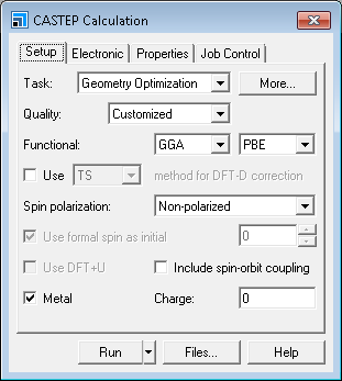
CASTEP Calculation dialog, Setup tab
Since you have already run a geometry optimization on the system, you only need to perform a single point energy calculation in order to obtain the density differences.
Change the Task to Energy.
On the Properties tab select the Electron density difference and select the Both atomic
densities and sets of atoms radio button. Ensure that you uncheck any other properties.
Click the Run button.
The job is submitted and begins to run. You should wait for it to complete before proceeding to the next section.
When the job has finished, you should save the project.
Select File | Save Project from the menu bar.
4. To display the fragment density difference
When the calculation finishes, you can display the charge density difference. Begin by closing all the open windows.
Select Window | Close All from the menu bar.
Now open the output structure for the job you just ran.
Open the document (1x1) CO on Pd (1 1 0).xsd in the folder (1x1) CO on Pd (1 1 0) CASTEP Energy.
Click the CASTEP button  on the Modules
toolbar and select Analysis.
on the Modules
toolbar and select Analysis.
Select the Electron density difference option, check the View isosurface on import checkbox and uncheck the
Use atomic densities checkbox. Click the Import button.
When you select Use atomic densities the density difference is computed with respect to atoms. When it is unchecked, the difference is computed with respect to fragments.
This displays an isosurface of the difference density at a value of about 0.1 electrons / Å3. Now you should create a more chemically useful isosurface.
Right-click on the document and select Display Style from the shortcut menu to open the Display Style dialog. On the Isosurface tab set the Isovalue to 0.05 and select +/- from the Type dropdown list.
This procedure displays two isosurfaces together. One is at a value of 0.05 and is colored blue, the other is at -0.05 and is colored yellow. The blue areas show where the electron density has been enriched with respect to the fragments. Conversely, the yellow areas show where the density has been depleted.
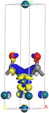
Charge density difference for CO Pd (110)
You can gain further insight into the changes in bonding by displaying the density difference as a 2D slice. You can do this using the Volume Visualization toolbar.
Select one of the isosurfaces and press DELETE.
The visibility of isosurfaces and slices can also be controlled, without deleting, using the Volumetric Selection dialog.
Select View | Toolbars | Volume Visualization from the menu bar.
Now use the Create Slices tool to create a 2D slice from the data.
Click the Create Slices arrow  tool and select Parallel to B & C Axis from the dropdown list.
Click on the 2D slice to select it, hold down the SHIFT and ALT keys and the right mouse
button to move the slice so that it cuts through the CO molecule.
You now have a 2D slice showing the density difference through the CO molecule. Next you will adjust the data range of the slice and change the color scheme to differentiate more easily between regions of electron depletion and electron enrichment.
Select the slice. Click the Color Maps button  on the Volume Visualization toolbar to open the Color Maps dialog.
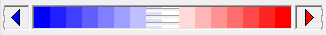
Change the Spectrum to Blue-White-Red, set From to -0.2
and To to 0.2, and set the value of Bands to 16.
Each of the 16 colors represents a specific range of the charge density. In this plot a loss of electrons is indicated in blue, while electron enrichment is indicated in red. White indicates regions with very little change in the electron density. You can see the red and blue areas more clearly if you hide the white areas.
Click on the two colors in the center of the selector on the Color Maps dialog.
The selector should now look like this:
The final image should resemble the one shown here:
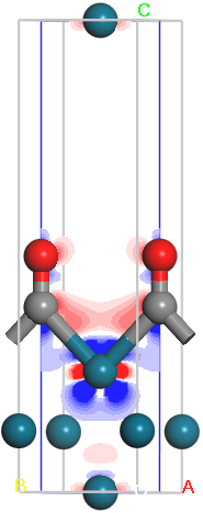
2D charge density difference for CO Pd (110)
Based on this, which atoms have lost electron density? Can you tell which orbitals lost electrons? Which orbitals on which atoms gained electrons? Does this match your expectations for carbon-metal bonding?
If you are interested you could repeat this section of the tutorial using the atomic density difference rather than the fragment density difference. Simply make sure that you check Use atomic densities when you import the density difference.
This is the end of the tutorial.