Adsorption of CO onto a Pd(110) surface

Purpose: Introduces the use of CASTEP for calculating the adsorption energy of a gas onto a metal surface.

Modules: Materials Visualizer, CASTEP

Time:   

Prerequisites: Using the crystal builder

Background

In this tutorial you will examine the adsorption of CO on Pd(110). The Pd surface plays a crucial role in a variety of catalytic reactions. Understanding how molecules interact with such surfaces is one of the first steps to understanding catalytic reactions. In this context, DFT simulations can contribute to this understanding by addressing the following questions:

• Where does the molecule want to adsorb?
• How many molecules will stick to the surface?
• What is the adsorption energy?
• What does the structure look like?
• What are the mechanisms of adsorption?

You will focus on one adsorption site, the short bridge site, as it is known to be energetically preferred at fixed coverage. At 1 ML coverage the CO molecules repel each other preventing them from aligning exactly perpendicular to the surface. You will calculate the energy contribution of this tilting to the chemisorption energy by considering a (1 × 1) and (2 × 1) surface unit cell.

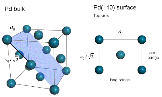
Pd bulk and a top view on the Pd(110) surface. The (110) cleave plane is highlighted in blue. a₀ is the bulk lattice constant, also known as the lattice parameter.

Introduction

In this tutorial, you will use CASTEP to optimize and calculate the total energies of several different systems. Once you have determined these energies, you will be able to calculate the chemisorption energy for CO on Pd(110).

This tutorial covers:

• Getting started
• To optimize bulk Pd
• To build and optimize CO
• To build the Pd(110) surface
• To relax the Pd(110) surface
• To add CO to the 1 × 1 Pd(110) surface and optimize the structure
• To set up and optimize the 2 × 1 Pd(110) surface
• To analyze the energies
• To analyze the density of states (DOS)

In order to ensure that you can follow this tutorial exactly as intended, you should use the Settings Organizer dialog to ensure that all your project settings are set to their BIOVIA default values. See the Creating a project tutorial for instructions on how to restore default project settings.

1. Getting started

Begin by starting Materials Studio and creating a new project.

Open the New Project dialog and enter CO_on_Pd as the project name, click the OK button.

The new project is created with CO_on_Pd listed in the Project Explorer.

This tutorial consists of five distinct calculations. To make it easier to manage your project, you should begin by preparing five subfolders in your project.

Right-click on the root icon in the Project Explorer and select New | Folder, repeat this four more times. Rename the folders Pd bulk, Pd(110), CO molecule, (1x1) CO on Pd(110) and (2x1) CO on Pd(110).

2. To optimize bulk Pd

The crystal structure of Pd is included in the structure library provided with Materials Studio.

In the Project Explorer, right-click on the Pd bulk folder and select Import... to open the Import Document dialog. Navigate to Structures/metals/pure-metals and import Pd.xsd.

The bulk Pd structure is displayed. You can change the display style to ball and stick.

Right-click in the Pd.xsd 3D Viewer and select Display Style to open the Display Style dialog. On the Atom tab, select Ball and stick and close the dialog.

Now optimize the geometry of the bulk Pd using CASTEP.

Click the CASTEP button on the Modules toolbar then select Calculation or select Modules | CASTEP | Calculation from the menu bar.

This opens the CASTEP Calculation dialog.

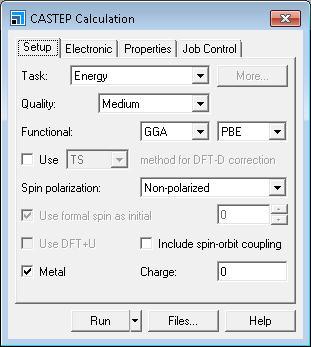
CASTEP Calculation dialog, Setup tab

Cell optimization of crystals requires more accurate calculations than those performed with default settings.

Change the Quality from Medium to Fine.

To maintain consistency across the calculations that you are going to perform, you should make some changes on the Electronic tab.

Select the Electronic tab and click the More... button to open the CASTEP Electronic Options dialog. On the Basis tab check the Use custom energy cutoff checkbox and make sure that the field value is 570.0 eV. This ensures that all calculations in the tutorial use the same energy cut-off.

The default values for geometry optimization do not include optimization of the cell.

Change the Task from Energy to Geometry Optimization. Click the More... button to open the CASTEP Geometry Optimization dialog. Select Full from the Cell optimization dropdown list and close the dialog.

Click the Run button. A message dialog about conversion to the primitive cell is displayed. Click the Yes button.

The job is submitted and starts to run. You should proceed to the next section and build the CO molecule but return here when the calculation is complete to display the Lattice Parameters.

When the job has finished, you must convert the primitive cell result back to a conventional cell representation in order to proceed with building the Pd(110) surface in step 4.

In the Project Explorer, open Pd.xsd located in the Pd CASTEP GeomOpt folder. Select Build | Symmetry | Conventional Cell from the menu bar.

You should now save your project files.

Select File | Save Project, then Window | Close All from the menu bar. In the Project Explorer, re-open the optimized Pd.xsd.

Right-click in the 3D Viewer and select Lattice Parameters.

This opens the Lattice Parameters dialog. The value of a should be approximately 3.962 Å, compared with the experimental value of 3.89 Å.

Close the Lattice Parameters dialog and Pd.xsd.

3. To build and optimize CO

CASTEP will only work with periodic systems. To optimize the geometry of the CO molecule, you must put it into a crystal lattice.

In the Project Explorer, right-click on the CO molecule folder and select New | 3D Atomistic Document. Rename the new document CO.xsd.

An empty 3D Viewer is displayed. You will use the Build Crystal tool to create an empty cell and then add the CO molecules to it.

Select Build | Crystals | Build Crystal... from the menu bar to open the Build Crystal dialog. Choose the Lattice Parameters tab and change each cell Length a, b, and c to 8.00. Click the Build button.

An empty cell is displayed in the 3D Viewer.

Select Build | Add Atoms from the menu bar to open the Add Atoms dialog.

The C-O bond length in the CO molecule has been determined experimentally as 1.1283 Å. By adding the atoms using Cartesian coordinates you can create your CO molecule with exactly this bond length.

Select the Options tab and ensure that the Coordinate system is set to Cartesian. On the Atoms tab click the Add button.

A carbon atom is added at the origin of the cell.

Change the Element to O, leave the x and y values as 0.000. Change the z value to 1.1283. Click the Add button and close the dialog.

You are now ready to optimize your CO molecule.

Open the CASTEP Calculation dialog.

The settings from the previous calculation have been retained. However, you do not need to optimize the cell for this calculation.

Open the CASTEP Geometry Optimization dialog. Select None from the Cell optimization dropdown list and close the dialog.

On the Properties tab of the CASTEP Calculation dialog check the Density of states checkbox. Change the k-point set to Gamma and check the Calculate PDOS checkbox. Click the Run button.

When asked about converting to higher symmetry, click the No button to proceed with the current symmetry.

The calculation starts. You can move onto building the Pd(110) surface as you will analyze the energy at the end of the tutorial.

4. To build the Pd(110) surface

This section of the tutorial uses the optimized Pd structure from the Pd bulk part of the tutorial.

Select File | Save Project, then Window | Close All from the menu bar. Open Pd.xsd in the Pd bulk/Pd CASTEP GeomOpt folder.

Creating the surface is a two step process. The first step is to cleave the surface and the second is to create a slab containing the surface and a region of vacuum.

Select Build | Surfaces | Cleave Surface from the menu bar to open the Cleave Surface dialog. Change the Cleave plane (h k l) from -1 0 0 to 1 1 0 and press TAB. Increase the Fractional Thickness to 1.5. Click the Cleave button and close the dialog.

A new 3D Viewer is opened containing the 2D periodic surface. However, CASTEP requires a 3D periodic system as input, this is obtained using the Vacuum Slab tool.

Select Build | Crystals | Build Vacuum Slab... from the menu bar to open the Build Vacuum Slab Crystal dialog. Change the Vacuum thickness from 10.00 to 8.00 and click the Build button.

The structure changes from 2D to 3D periodic and a vacuum is added above the atoms. Before continuing, you must reorient the lattice.

Open the Lattice Parameters dialog and select the Advanced tab, click the Re-orient to standard button. Close the dialog.

You should also change the lattice display style and rotate the structure so that the z-axis is vertical on the screen.

Open the Display Style dialog and select the Lattice tab. In the Display style section, change the Style from Default to Original. Close the dialog.

Press the UP arrow key twice.

The 3D view shown below is displayed:

The Pd atom with the largest z-coordinate will be called "the uppermost Pd layer".

Later in this tutorial, you will need to know the bulk interlayer spacing d_o. You can calculate this using the atom coordinates.

Select View | Explorers | Properties Explorer from the menu bar. Select the Pd atom with FractionalXYZ x = 0.5 and y = 0.5. Note the z value of this atom from the XYZ property.

The z value should be 1.401 Å and this is the interlayer spacing. This z value refers to the Z coordinate from the (Cartesian) XYZ property and not FractionalXYZ.

For an fcc(110) system, d₀ can be calculated as:

Before you relax the surface, you must constrain the Pd atoms in the bulk as you only need to relax the surface.

Hold down SHIFT and select all the Pd atoms except the uppermost Pd layer. Select Modify | Constraints from the menu bar to open the Edit Constraints dialog. Check the Fix fractional position checkbox and close the dialog.

The bulk atoms have been constrained. You can see the constrained atoms by changing their display color.

In the 3D Viewer, click anywhere to deselect the atoms. Open the Display Style dialog and select the Atom tab. Change the Color by option to Constraint.

This 3D view is now displayed:

Change the Color by option back to Element and close the dialog.

This structure is needed for the Pd(110) surface relaxation and also as a starting model for (1x1) CO on Pd(110) optimization.

Select File | Save As... from the menu bar. Navigate to the Pd(110) folder and click the Save button.

Hold down CTRL and drag the document into the (1x1) CO on Pd(110) folder. Rename the document (1x1) CO on Pd(110).

Select File | Save Project, then Window | Close All from the menu bar.

5. To relax the Pd(110) surface

Now you are ready to optimize the Pd (110) surface.

From the Project Explorer, open Pd (1 1 0).xsd in the Pd(110) folder. Open the CASTEP Calculation dialog and then the CASTEP Geometry Optimization dialog. Ensure that Cell optimization is set to None and close the dialog.

You should also calculate the density of states for the system.

Select the Properties tab on the CASTEP Calculation dialog. Check the Density of states and Calculate PDOS checkboxes and change the k-point set to Fine.

You are ready to run the calculation.

Click the Run button and close the CASTEP Calculation dialog.

When asked about converting to higher symmetry, click the No button to proceed with the current symmetry.

The calculation will take some time to run and so you will perform the analysis at the end. You should move on and construct the next set of surfaces.

Select File | Save Project then Window | Close All from the menu bar.

6. To add CO to the 1 × 1 Pd(110) surface and optimize the structure

Now you are going to work with the structure in the (1x1) Co on Pd(110) folder.

In the Project Explorer, open (1x1) CO on Pd(110).xsd in the (1x1) CO on Pd(110) folder.

Now add the CO molecule above the short bridge position. You will make use of the fact that for CO on Pd(110), bond lengths have been experimentally determined.

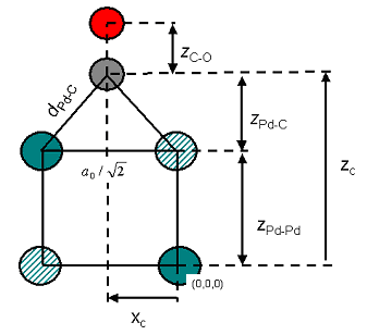
Geometry of CO on Pd(110) in the yz-plane. Hatched atoms are not displayed in Lattice: Original display mode.

The first step is to add the carbon atom. The Pd-C bond length (denoted above as d_Pd-C) should be 1.93 Å. When you use the Add Atom tool you can enter either Cartesian or fractional coordinates but in this case you will use fractional coordinates, x_C, y_C, and z_C. x_C and y_C are simple as y_C = 0.5 and x_C = 0. However, determination of z_C is slightly more difficult. You will construct it from the two distances z_Pd-C and z_Pd-Pd.

z_Pd-Pd is simply the lattice parameter a₀ divided by √2 (it should be 2.80 Å).

z_Pd-C is obtained from the formula:

It should be 1.33 Å.

Add z_Pd-C and z_Pd-Pd to obtain z_C (it should be 4.13 Å). Now convert this distance into a fractional length. You do this using the Lattice parameters.

Right-click in the 3D Viewer and select Lattice Parameters from the shortcut menu. Note the value of c.

To calculate the fractional z coordinate, you divide z_C by the c lattice parameter (you should obtain 0.382).

Open the Add Atoms dialog and choose the Options tab. Check that the Coordinate system is Fractional. On the Atoms tab change the Element to C, change a to 0.0, b to 0.5, and c to 0.382. Click the Add button.

If you want to confirm that you have set up the model correctly, use the Measure/Change tool.

Click the Measure/Change arrow on the toolbar and select Distance from the dropdown list. Click on the Pd-C bond.

The next step is to add the oxygen atom.

On the Add Atoms dialog, change the Element to O.

Experimentally, the C-O bond length has been determined as 1.15 Å. In fractional coordinates this is 0.107, adding this value to the fractional z-coordinate of carbon (0.382), the z-coordinate of oxygen is 0.489.

Change the value of c to 0.489 and click the Add button. Close the dialog.

The calculations for the Pd surface model were carried out using P1 symmetry. However, the system has a higher symmetry, even after the addition of the CO molecule. You can find and impose symmetry, using the Find Symmetry tool, to speed up further calculations.

Click the Find Symmetry button on the Symmetry toolbar to open the Find Symmetry dialog. Click the Find Symmetry button then the Impose Symmetry button.

The symmetry is PMM2.

Open the Display Style dialog and select the Lattice tab. Change the Style to Default. On the Atom tab, select the Ball and stick display style and close the dialog.

The structure should look similar to this:

Before you optimize the geometry of the structure, you should save it in the (2x1) CO on Pd(110) folder.

Select File | Save from the menu bar to save the 1x1 system. Then also select File | Save As... from the menu bar, navigate to the (2x1) CO on Pd(110) folder and save the document as (2x1) CO on Pd(110).xsd.

You are now ready to optimize the structure.

Select File | Save Project, then Window | Close All from the menu bar.

In the Project Explorer, open (1x1)CO on Pd(110).xsd in the (1x1)CO on Pd(110) folder.

Open the CASTEP Calculation dialog.

The parameters from the previous calculation should have been retained.

Click the Run button and close the dialog.

Once again, you can move onto building the final structure while the calculation progresses.

7. Setting up and optimizing the 2 × 1 Pd(110) surface

The first step is to open the 3D Atomistic document in the (2 × 1) CO on Pd(110) folder.

In the Project Explorer, open (2x1) CO on Pd(110).xsd in the (2x1) CO on Pd(110) folder.

This is currently a 1 × 1 cell so you need to use the Supercell tool to change it to a 2 × 1 cell.

Select Build | Symmetry | Supercell from the menu bar to open the Supercell dialog. Increase B to 2 and click the Create Supercell button and close the dialog.

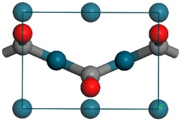
The structure should look like this:

(2 × 1) Cell of CO on Pd(110)

Now tilt the CO molecules with respect to each other. To simplify this operation, identify the CO molecule at y = 0.5 as molecule A and the one at y = 0.0 as molecule B.

Select the carbon atom of molecule B. In the Properties Explorer, open the XYZ property and subtract 0.6 from the X field. Repeat this for the oxygen atom of molecule B but subtract 1.2 from the X field.

Now repeat this for molecule A.

Select the carbon atom of molecule A. In the Properties Explorer, open the XYZ property and add 0.6 to the X field. Repeat this for the oxygen atom of molecule A but add 1.2 to the X field.

The view down the z-axis of the molecule should look like this:

However, you will notice that the Pd-C and C-O bond lengths have changed from their original values.

Select the carbon atom in molecule A and use the Properties Explorer to change the Z field of the FractionalXYZ property to 0.369. Repeat this for molecule B.

This corrects the Pd-C bond length. You can use the Measure/Change tool to correct the C-O bond length.

Click the Measure/Change button on the Sketch toolbar and select Distance from the dropdown list. Click on the C-O bond for molecule A.

Choose the 3D Viewer Selection Mode tool on the 3D Viewer toolbar and select the monitor. In the Properties Explorer, change the Filter to Distance.

Change the Distance property to 1.15 Å. Repeat this for molecule B.

Now recalculate the symmetry of the system.

Open the Find Symmetry dialog and click the Find Symmetry button then the Impose Symmetry button.

The symmetry is PMA2. The view of the unit cell changes from 3 CO molecules on the Pd surface to only 2. You are now ready to optimize the geometry of your system.

Open the CASTEP Calculation dialog and click Run.

The calculation starts. When the calculation finishes, you will need to extract the total energy of the system as detailed in the next section. You can move onto the next section to extract the energies from the previous calculations.

8. To analyze the energies

In this section you are going to calculate the chemisorption energy ΔE_chem. This is defined as:

Allowing the CO atoms to tilt against each other, hence reducing the self repulsion of the CO molecules, should result in a gain in energy. The repulsion energy can be calculated from:

To calculate these properties, you need to extract the total energies from CASTEP text output documents for each simulation.

In the Project Explorer, open CO.castep in the CO molecule/CO CASTEP GeomOpt folder. Press CTRL + F and search for Final Enthalpy. Note down the value that appears in that line. Repeat the procedure to find the total energies of the other systems and so complete the table.

Simulation	Total Energy (eV)
CO molecule
Pd(110)
(1×1)CO on Pd(110)
(2×1)CO on Pd(110)

Once you have the energies, simply use the above equations to calculate ΔE_chem and ΔE_rep. These should have values of approximately -1.79 eV and  -0.06 eV, respectively.

9. To analyze the density of states (DOS)

Next, you will examine the changes in the density of states (DOS). This will allow you to obtain an insight into the bonding mechanism of CO on Pd(110). To do this, you need to display the density of states of the isolated CO molecule and of (2x1) CO on Pd(110).

In the Project Explorer, open CO.xsd in the CO molecule/CO CASTEP GeomOpt folder.

Click the CASTEP button on the Modules toolbar, then select Analysis to open the CASTEP Analysis dialog.

Select the Density of states. Click the Partial radio button and uncheck the f and Sum checkboxes. Click the View button.

A chart document is displayed showing the PDOS for the CO molecule.

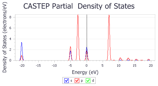
PDOS of CO molecule

Repeat the above for (2x1) CO on Pd(110).xsd.

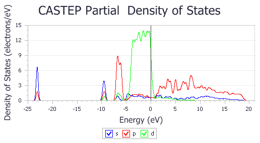
PDOS of (2x1) CO on Pd(110)

It is clear that the electronic states of the isolated CO molecule at approximately -20, -5, and -2.5 eV are considerably lowered in energy as the CO binds to the surface.

The default pseudopotential for Pd, Pd_2017R2.otfg, treats 4s and 4p semicore states as valence. This results in sharp peaks in the calculated DOS at about -84 and -49 eV. The chart above excludes those states; this can be achieved by using Properties Explorer to change the maximum and minimum values along X and Y axes.

As an independent exercise you can analyze PDOS further by investigating contributions to the PDOS of the adsorbate complex that arise from the C and O atoms.

Hold down SHIFT and select all C and O atoms in the (2x1) CO on Pd(110).xsd document. Generate partial DOS as described above - the chart shows the effect of hybridization with Pd states which manifests itself as broadening of the energy levels and their general shift towards lower energies.

There are a number of additional experiments that can be carried out as an independent exercise, for example:

• Investigate the accuracy of the results by checking convergence with respect to calculation parameters:
  1. Repeat the chemisorption calculation with a significantly higher value for the vacuum thickness (for example, 15 Å instead of 8 Å).
  2. Repeat the chemisorption calculation with a more accurate k-point sampling; on the CASTEP Electronic Options dialog, k-points tab, use a Separation of 0.03 1/Å to produce a denser k-point grid. This step can be repeated with few more values until the chemisorption energy is converged to the desired accuracy.
  3. Similar to the previous step, repeat the calculations by increasing the energy cutoff on the CASTEP Electronic Options dialog, Basis tab; check Use custom energy cutoff to enable this step.

• The number of substrate layers can affect the result substantially; you can repeat this tutorial with more Pd layers by using a higher value for the Fractional Thickness when generating the surface.
• Surface calculations in a slab geometry often benefit from application of a dipole correction, especially when there is a pronounced dipole moment - as in the CO molecule.

  CASTEP allows you to apply such a correction by selecting a Self-consistent option for the Apply dipole correction on the CASTEP Electronic Options dialog, SCF tab. Repeat calculations with this setting to check whether it affects the energetics of CO adsorption.

  It is recommended to use the All Bands/EDFT option for the Electronic minimizer setting in this tutorial (on the SCF tab of the CASTEP Electronic Options dialog). The default Density Mixing option exhibits convergence problems for the elongated thin cells that are used in these calculations.

  You could additionally examine electrostatic potential by using the Potentials selection on the CASTEP Analysis dialog. A chart of the average profile of the electrostatic potential will be created when the Import button is clicked.

  There is a difference between the charts generated for calculations with and without a dipole correction applied.

Vacuum width has to be greater than 8 Å in order to generate the chart of electrostatic potential, so this last exercise can be performed only by increasing the vacuum thickness.

This is the end of the tutorial.