Example - A Bulk Terminated Silicon Surface

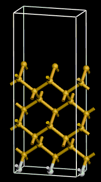
When the supercell does not have full 3D periodicity the calculation must be converged with respect to other supercell parameters. Consider a surface. We will use the Si(100) surface reconstruction as an example. Figure 5 below shows the bulk terminated Si(100) surface.

Figure 5: The bulk terminated Si(100) surface

In one direction we have a defect; after some point there will be a complete absence of atoms, essentially out to infinity. In the opposite direction we move into the bulk and in principle we should include an infinite number of bulk layers below the top few surface layers.

Both of these requirements are computationally impractical. In practice we must include just enough bulk layers so that the inner bulk atoms remain in place during the calculation and only the top surface layers reconstruct.Also, only a finite amount of vacuum space above the top surface layer is practical. However, when a supercell is repeated periodically in all three spatial directions the bottom bulk-like region of one supercell borders upon the top vacuum region of the supercell below it (figure 6). If the vacuum region is not thick enough the uncompensated charges on the bottom of the one supercell and the top of the supercell under it will cause an unphysical interaction. Vertically adjacent supercells must not be able to 'see' one another.

Figure 6: A finite vacuum gap may cause an interaction between neighbouring atomic layers in vertically adjacent supercells

Other effects are caused by uncompensated charges. The bottom layer of the supercell, which should be bulk-like, may reconstruct. To prevent this we can constrain these atoms to remain in their bulk positions. Another effect is an interaction between the top surface layer uncompensated charges and the bottom layer uncompensated charges through the intermediate layers. The supercell must contain sufficient numbers of layers of atoms to space the top and bottom layers out so as to minimise the internal interactions in the supercell. A neat trick is to use hydrogen passivation. In this the dangling bonds of the bottom bulk like layers are compensated by bonding these atoms to hydrogen atoms. This introduces extra atoms into the calculation but reduces the overall number of atoms needed because the number of spacer layers in the supercell is reduced (also, hydrogen is computationally cheap). The thickness of the vacuum gap can also be reduced when hydrogen passivation is used (remember empty space is a computational expense too).

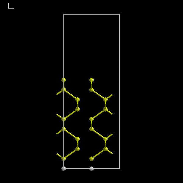
The Si(100) surface is known to have a simple 2x1 dimerised structure. The small in-plane unit cell of the reconstructed surface means that we can use a small supercell and we do not need many atoms. The following initial supercell will be sufficient (figure 7). Notice the hydrogen passivation.

Figure 7: A hydrogen passivated Si(100) supercell with a 7 Å vacuum gap and 9 layers of silicon.

This is a crucial feature of performing geometry optimisation on surfaces. The initial surface unit cell must be large enough to enclose any expected reconstruction. A Si(111)-1x1 supercell will not reconstruct into the Si(111)-7x7 Takayanagi reconstruction! If no suggestions have been provided as to possible reconstructed periodicities by previous theoretical or experimental work then the user might have to begin with a large supercell and perform a variable cell calculation (in case of lateral relaxations).

Now we must perform the abovementioned supercell convergence checks. We will use a 9 k-point MP grid with a cutoff energy of 260eV for this (we will converge our calculation with respect to basis set parameters later). Let us start with a large vacuum gap of 15Å (I know that this is entirely sufficient from experience). We will now be able to perform several calculations with 7, 8, 9, 10 and 11 layers of silicon and not have to worry about the vacuum gap - one problem at a time. The supercell lattice matrix and the atomic coordinate list in the .cell file for 7 layers of silicon looks like

	%BLOCK LATTICE_CART
  		7.6801695932    0.0000000000    0.0000000000
    		0.0000000000    3.8801700000    0.0000000000
    		0.0000000000    0.0000000000   24.5037250000
	%ENDBLOCK LATTICE_CART

	%BLOCK POSITIONS_FRAC
    		H    0.2500000000   -0.0103307854   -0.0000000000
    		H    0.7500000000   -0.0103307854   -0.0000000000
    	       Si    0.5000000000    0.9896692146    0.1662206460
    	       Si    0.5000000000    0.9896692146    0.3878481741
    	       Si    0.2500000000    0.4948346073    0.0554068820
    	       Si    0.2500000000    0.4948346073    0.2770344101
    	       Si    0.7500000000    0.4948346073    0.0554068820
    	       Si    0.7500000000    0.4948346073    0.2770344101
    	       Si    0.0000000000    0.9896692146    0.1662206460
    	       Si    0.0000000000    0.9896692146    0.3878481741
   	       Si   -0.0000000000    0.4948346073    0.1108137640
    	       Si   -0.0000000000    0.4948346073    0.3324412921
    	       Si    0.7500000000    0.9896692146    0.2216275281
    	       Si    0.5000000000    0.4948346073    0.1108137640
    	       Si    0.5000000000    0.4948346073    0.3324412921
    	       Si    0.2500000000    0.9896692146    0.2216275281
	%ENDBLOCK POSITIONS_FRAC

Notice the hydrogen atoms. Now for the constraints on the bottom layer silicon atoms and the hydrogen atoms (the H atoms must also be constrained because the have a tendency to move into awkward formations). The list of constraints whose format was specified before looks like

	%BLOCK IONIC_CONSTRAINTS
 		1    H   1    1.00000000    0.00000000    0.00000000
       		2    H   1    0.00000000    1.00000000    0.00000000
		3    H   1    0.00000000    0.00000000    1.00000000
 		4    H   2    1.00000000    0.00000000    0.00000000
       		5    H   2    0.00000000    1.00000000    0.00000000
       		6    H   2    0.00000000    0.00000000    1.00000000
  		7   Si   3    1.00000000    0.00000000    0.00000000
       		8   Si   3    0.00000000    1.00000000    0.00000000
       		9   Si   3    0.00000000    0.00000000    1.00000000
       	       10   Si   5    1.00000000    0.00000000    0.00000000
       	       11   Si   5    0.00000000    1.00000000    0.00000000
       	       12   Si   5    0.00000000    0.00000000    1.00000000
	%ENDBLOCK IONIC_CONSTRAINTS

NB You will also need to add some other settings to your cell file, especially

        fix_com = FALSE
        fix_all_cell = TRUE
        fix_all_ions = FALSE

as otherwise these constraints will interfere. See the ionic constraints section for more details.

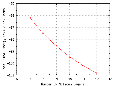
So now we have our supercells ready to run. The calculations were performed on 9 nodes of a Beowulf cluster. The total final energy per supercell atom as a function of the number of layers of silicon is shown in figure 8 below

Figure 8: The total final energy per supercell atom as a function of the number of layers of silicon.

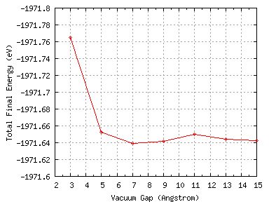
We can see that the energy per atom is decreasing almost linearly with the number of layers. We would need to add very many layers for the energy to not vary by the inclusion of more layers. We will use 9 layers of silicon in future calculations. With 9 silicon layers the vacuum gap was varied from 3 Å to 15 Å in 2 Å steps. The total final energy as a function of vacuum gap separation is shown below.

Figure 9: The total final energy as a function of the vacuum gap thickness

We can see that the total energy is converged with respect to the vacuum gap when this has a thickness greater than about 7 Å (there is a slight upwards kink after this). We will use a 9 Å vacuum gap in all future calculations.

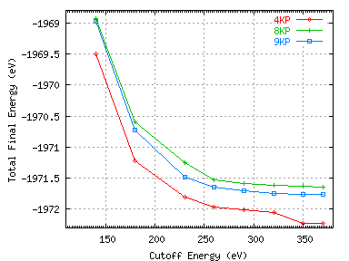
Now it remains to converge the basis set paramters. Cutoff energies of 140, 180, 230, 260, 290, 320, 350, and 370eV were used with MP grids containing 4, 8 and 9 k-points. The calculations were performed on a Beowulf cluster using 8 nodes for the 4 and 8 k-point calculations and 9 nodes for the 9 k-point calculation. The convergence of the total energy with basis set parameters is shown below.

Figure 10: Convergence of the total energy with respect to the basis set parameters

We can see that using 9 layers of silicon, a 9 Å vacuum gap, 9 k-points and a 370 eV cutoff energy will ensure minimisation of systematic errors with respect to both supercell aperiodicity and the basis set repectively.

So what results do we get? Click on the movie below to see the evolution of the atomic positions as the calculation progresses. Please use the 'back' button to close the movie.

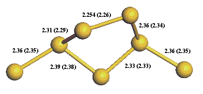
We can see that the result is an initial vertical relaxation followed by asymmetric dimerisation of the top layer silicon atoms. Asymmetric dimerisation has been seen experimentally [6] and has been confirmed by detailed theoretical calculations [7]. The bond lengths are shown in figure 11 below (the numbers in brackets are taken from reference [7]).

Figure 11: Principle bond lengths compared with the results of other theoretical work (in brackets).

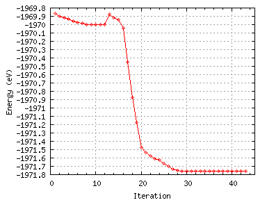
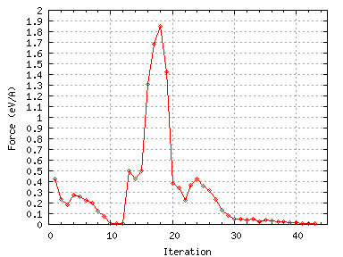
It is interesting to look at the evolution of the total energy and the forces as the calculation progresses. Figures 12 and 13 below shows this.

Figure 12: The variation of the total energy with BFGS iteration number.

Figure 13: The variation of the maximum force with BFGS iteration number.

There is an inital dip in the forces at around iteration 14 as some search direction is tried but this causes an increase in the energy. Then there is a large increase in the forces (presumably due due dimer attraction) accompanied by a large energy gain which are due to dimerisation. There is then a small peak in the forces and the energy at about iteration 24 as the energy barrier to asymmetric dimerisation is overcome.

In summary, this example has illustrated the use of constraints upon atomic positions and has also looked at hydogen passivation and the variation of both the number of layers of atoms and the thickness of the vacuum gap as ways to deal with aperiodic supercell configurations such as surfaces.