Optical properties
Definition of optical constants
CASTEP can calculate the optical properties of solids that are due to electronic transitions.
In general, the difference in the propagation of an electromagnetic wave through vacuum and some other material can be described by a complex refractive index, N:

In vacuum N is real, and equal to unity. For transparent materials it is purely real, the imaginary part being related to the absorption coefficient by:

The absorption coefficient indicates the fraction of energy lost by the wave when it passes through the material, so that the intensity at the distance x from the surface is:

where I(0) is the intensity of the incident light.
The reflection coefficient can be obtained for the simple case of normal incidence onto a plane surface by matching both the electric and magnetic fields at the surface:

However, when performing calculations of optical properties it is common to evaluate the complex dielectric constant and then express other properties in terms of it. The complex dielectric constant, ε(ω), is given by:

and hence the relation between the real and imaginary parts of the refractive index and dielectric constant is:

Another frequently used quantity for expressing optical properties is the optical conductivity, σ(ω):

Optical conductivity is usually used to characterize metals, however CASTEP is aimed more toward the optical properties of insulators and semiconductors. The main difference between the two is that intraband transitions play important role in the IR part of the optical spectra of metals and these transitions are not considered at all in CASTEP.
A further property that can be calculated from the complex dielectric constant is the energy loss function. It describes the energy lost by an electron passing through a homogeneous dielectric material and is given by:

Connection to experimental observables
Experimentally, the most accessible optical parameters are the absorption, η(ω), and the reflection, R(ω), coefficients. In principle, given the knowledge of both of these, the real and imaginary parts of N can be determined, through Eq. CASTEP 49 and Eq. CASTEP 50. Eq. CASTEP 51 allows expression in terms of the complex dielectric constant. However, in practice, the experiments are more complicated than the case of normal incidence considered above. Polarization effects must be accounted for and the geometry can become quite complex (for example, transmission through multilayered films or incidence at a general angle).
CASTEP supports spin-polarized calculations of optical properties for magnetic systems. Only transitions between the states with the same spin are allowed. For a more general discussion of the analysis of optical data see Palik (1985).
Connection to electronic structure
The interaction of a photon with the electrons in the system is described in terms of time dependent perturbations of the ground state electronic states. Currently CASTEP provides two approaches to optical properties calculations; one is based on standard DFT Kohn-Sham orbitals and the other uses more accurate but much more time-consuming time-dependent DFT (TD-DFT) theory.
DFT optics
In this approach excited states are represented as unoccupied Kohn-Sham states. Transitions between occupied and unoccupied states are caused by the electric field of the photon (the magnetic field effect is weaker by a factor of v/c). When these excitations are collective they are known as plasmons (which are most easily observed by the passing of a fast electron through the system rather than a photon, in a technique known as Electron Energy Loss Spectroscopy, described by Eq. CASTEP 54 , since transverse photons do not excite longitudinal plasmons). When the transitions are independent they are known as single particle excitations. The spectra resulting from these excitations can be thought of as a joint density of states between the valence and conduction bands, weighted by appropriate matrix elements (introducing selection rules).
Evaluation of the dielectric constant
CASTEP calculates the imaginary part of the dielectric constant, which is given by:

where u is the vector defining the polarization of the incident electric field.
This expression is similar to Fermi's Golden rule for time dependent perturbations, and ε2(ω) can be thought of as detailing the real transitions between occupied and unoccupied electronic states. Since the dielectric constant describes a causal response, the real and imaginary parts are linked by a Kramers-Kronig transform. This transform is used to obtain the real part of the dielectric function, ε1(ω).
Details of the calculation
Evaluation of matrix elements
The matrix elements of the position operator that are required to describe the electronic transitions in Eq. CASTEP 55 may normally be written as matrix elements of the momentum operator allowing straightforward calculation in reciprocal space. However, this depends on the use of local potentials (Read and Needs, 1991), while in CASTEP nonlocal potentials are more often used. The corrected form of the matrix elements is:

Ultrasoft pseudopotentials produce an additional contribution to optical matrix elements that is also included in CASTEP results.
Drude correction
The intraband contribution to the optical properties affects mainly the low energy infrared part of the spectra. It can be described sufficiently accurately using a semiempirical Drude term in the optical conductivity:

in terms of the plasma frequency ωP and damping parameter γD which depends on many details of the material and is usually obtained from experiment. The Drude damping parameter describes the broadening of the spectra due to effects not included in the calculation. Examples of processes that contribute to this broadening are electron-electron scattering (including Auger processes), electron-phonon scattering, and electron-defect scattering. This last contribution is usually the most important. As a result an a priori determination of the broadening would require knowledge as to the concentrations and kinds of defects present in the sample under study.
Polarization
For materials that do not display full cubic symmetry, the optical properties will display some anisotropy. This can be included in the calculations by taking the polarization of the electromagnetic field into account. As mentioned above, the unit vector u defines the polarization direction of the electric field. When evaluating the dielectric constant there are three options:
- polarized: requires a vector to define the direction of the electric field vector for the light at normal incidence to the crystal.
- unpolarized: requires a vector to define the direction of propagation of incident light at normal incidence to the crystal. The electric field vector is taken as an average over the plane perpendicular to this direction.
- polycrystal: no direction need be specified, the electric field vectors are taken as a fully isotropic average.
Scissors operator
As discussed below, the relative position of the conduction to valence bands is erroneous when the Kohn-Sham eigenvalues are used. In an attempt to fix this problem, inherent in DFT, a rigid shift of the conduction band with respect to the valence band is allowed. This procedure of artificially increasing the band gap is know as a scissor operator.
Limitations of the method
Local field effects
The level of approximation used here does not take any local field effects into account. These arise from the fact that the electric field experienced at a particular site in the system is screened by the polarizability of the system itself. So, the local field is different from the applied external field (that is, the photon electric field). This can have a significant effect on the spectra calculated (see the example of bulk silicon calculation below) but it is prohibitively expensive to calculate for general systems at present.
Quasiparticles and the DFT bandgap
In order to calculate any spectral properties it is necessary to identify the Kohn-Sham eigenvalues with quasiparticle energies. Although there is no formal connection between the two, the similarities between the Schrödinger-like equation for the quasiparticles and the Kohn-Sham equations allow the two to be identified. For semiconductors, it has been shown computationally (by comparing GW and DFT band structures) that most of the difference between Kohn-Sham eigenvalues and the true excitation energies can be accounted for by a rigid shift of the conduction band upward with respect to the valence band (Godby et al., 1992). This is attributed to a discontinuity in the exchange-correlation potential as the system goes from (N)-electrons to (N+1)-electrons during the excitation process. There can, in some systems, be considerable dispersion of this shift across the Brillouin zone, and the scissor operator used here will be insufficient.
Excitonic effects
In connection with the absence of local field effects, excitonic effects are not treated in the present formalism. This will be of particular importance for ionic crystals (for example NaCl) where such effects are well known.
Other limitations
- The nonlocal nature of the GGA exchange-correlation functionals is not taken into account when evaluating the matrix elements but it is expected that this will have a small effect on the calculated spectra.
- Phonons and their optical effects have been neglected.
- Finally, there is an intrinsic error in the matrix elements for optical transition due to the fact that pseudowavefunctions have been used (that is they deviate from the true wavefunctions in the core region). However, the selection rules will not be changed when going from pseudo- to all-electron wavefunctions.
Sensitivity of optical properties to calculation parameters
Number of conduction bands
This parameter defines the energy range covered in the calculation, and it also determines the accuracy of the Kramers-Kronig transform. It is clear from Figure 1 that ε2(ω) converges rapidly with the number of conduction bands included.
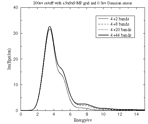
Figure 1. Convergence of the dielectric function with the number of conduction bands
Energy cutoff
The value of the energy cutoff that was used in the original SCF calculation of the ground state electron density is an important factor that determines the accuracy of the calculated optical properties. A bigger basis set provides more accurate self-consistent charge density and more variational freedom when searching for wavefunctions of unoccupied states. Figure 2 shows that while it is important to converge the calculation with respect to the planewave cutoff to obtain the correct energies for the spectral features, the shape of those features is reached rapidly.
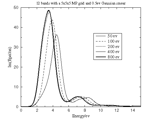
Figure 2. Convergence of the dielectric function with the cutoff energy
Number of k-points in the SCF calculation
The accuracy of the ground state electron density depends on the number of k-points used in the SCF run as well as on the basis set quality. Figure 3 reveals that the optical properties converge rapidly with the number of k-points used in the SCF run, which implies low sensitivity to the details of the charge density.
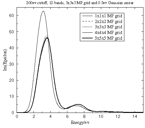
Figure 3. Convergence of the dielectric function with the number of k-points in the SCF calculation
Number of k-points for Brillouin zone integration
It is important to use a sufficient number of k-points in the Brillouin zone when running optical matrix element calculations. The matrix element changes more rapidly within the Brillouin zone than electronic energies themselves. Therefore, one requires more k-points to integrate this property accurately than are needed for an ordinary SCF calculation. Figure 4 clearly demonstrates the importance of converging the Brillouin zone integration for the optical properties with respect to the k-point density. Both energies and spectral features are strongly affected by the accuracy of this integration.
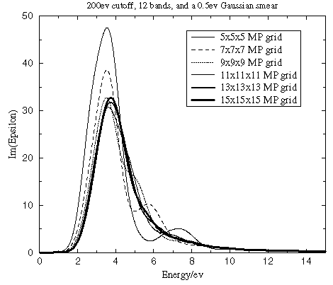
Figure 4. Convergence of the dielectric function with the number of k-points in the optical matrix elements calculation
TD-DFT optics
TD-DFT is a formally exact treatment of electronic excited states. The implementation in CASTEP follows the work of Hutter (2003), which takes a linear response approach to computing excitation energies directly. A benefit of this method is that the response wavefunctions for excited states are calculated and can then be used to derive further properties such as optical matrix elements and atomic forces. In the case of atomic forces, a geometry optimization or molecular dynamics run can be performed for a chosen excitation.
Hutter reformulated the equations of time-dependent Hartree-Fock in the Tamm-Dancoff approximation applied to TD-DFT (Hirata and Head-Gordon, 1999) so that they could be efficiently implemented in a plane-wave basis set. This self-consistent eigenvalue problem is solved in CASTEP by the user’s choice of conjugate gradient or block-Davidson minimizers. The result is a set of electronic excitation energies and linear response wavefunctions.
A technical report on the implementation details of the TD-DFT minimizers can be found at http://www.hector.ac.uk/cse/distributedcse/reports/castep02/.
A second report on the implementation of excited state forces can be found at http://www.hector.ac.uk/cse/distributedcse/reports/castep03/.